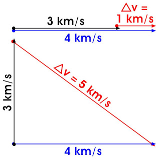
Rockets don't got a "range" like a car running out of gasoline. Instead they have "maximum velocity" called "Delta V".
A rocket's propellant tanks are like a "wallet" full of delta-V "money"
Each rocket maneuver has a delta-V "cost" which has to be paid with delta-V money. Don't have enough in your wallet? Then you can't afford to do that manuever.
A space mission is composed of several manuevers, each with a delta-V cost. The total is the delta-V mission cost.
Refilling the propellant tank is like putting more money in the wallet. This is why rocket engineers are trying to figure out how to put gasoline stations in space. Because it sucks trying to do a long trip in your car on one tank.
Most rockets are poor, with very little money in their wallet. So they can only afford the cheapest maneuvers
One of the cheapest maneuvers is called a "Hohmann transfer." Using one to go from Terra to Mars takes about 5,700 meters per second of delta-V money and 8.6 months of travel time. And about the same to return home.
Also you can't just take off on a Mars Hohmann any time you want. Terra and Mars have to be in the proper spots, which happens every 26 months. This is called a "Hohmann Launch Window." And once you reach Mars you have to wait 15.3 months before the return launch window happens.
The main way to get a handle on your ship definition is to decide what kinds of missions it will be capable of. Let's decide that the Solar Guard cruiser Polaris will be capable of taking off from Terra, travelling to Mars, landing on Mars, taking off from Mars, travelling to Terra, and landing on Terra. All without re-fuelling.
Keep in mind that this is an incredibly silly sort of ship to design. Any real spacecraft designer would design two craft: one surface to orbit shuttle, and one orbit to orbit vehicle.
Delta-V
Artwork by John Polgreen
RocketCat sez
All those cute starship spec sheets you see with moronic entries like "range" or "maximum distance" betray a dire lack of spaceflight knowledge. Spacecraft ain't automobiles, if they run out of gas they don't drift to a halt. DeltaV is the key.
The main number of interest is deltaV. This means "change of velocity" and is usually measured in meters per second (m/s) or kilometers per second (km/s). A spacecraft's maximum deltaV can be though of as how fast it will wind up traveling at if it keeps thrusting until the propellant tanks are dry.
If that means nothing to you, don't worry. The important thing is that a "mission" can be rated according to how much deltaV is required. For instance: lift off from Terra, Hohmann orbit to Mars, and Mars landing, is a mission which would take a deltaV of about 18,290 m/s. If the spacecraft
has equal or more deltaV capacity than the mission, it is capable of performing that mission.
The sum of all the deltaV requirements in a mission is called the deltaV budget.
This is why it makes sense to describe a ship's performance in terms of its total deltaV capacity, instead of its "range" or some other factor equally silly and meaningless. In Michael McCollum's classic Antares Dawn, when the captain asks the helmsman how much propellant they have, the helmsman replies that they have only 2200 kps (kilometers per second) left in the tanks.
The basic deltaV cost for liftoff and landing is what is needed to achieve orbital (or circular) velocity.
For a back-of-the-envelope calculation, figure boosting from Terra's surface into LEO will require about 9,400 m/s of deltaV. For other planets use the equation:
Δvo = sqrt[ (G * Pm) / Pr ]
where:
Δvo = deltaV to lift off into orbit or land on a planet from orbit (m/s)
Mercury's mass is 3.302e23 kg and radius is 2.439e6 m. sqrt[ (6.673e-11 * 3.302e23) / 2.439e6] = 3006 m/s liftoff deltaV.
Δvo is what you will use for missions like the Space Shuttle, where you just climb into orbit, deliver or pick up something, then land from orbit. However, if the mission involved travelling to other planets, you will have to use Δesc instead. This is "escape velocity", and is also the delta V required to land from deep space instead of landing from orbit.
Δesc = sqrt[ (2 * G * Pm) / Pr ]
Δesc = sqrt[ (1.3346e-10 * Pm) / Pr ]
where:
Δesc = deltaV for escape velocity from a planet (m/s)
Mercury's mass is 3.302e23 kg and radius is 2.439e6 m. sqrt[ (1.3346e-10 * 3.302e23) / 2.439e6] = 4251 m/s escape velocity deltaV.
So for our Polaris mission, basic deltaV for Terra escape or capture: 11,180 m/s, basic deltaV for Mars escape or capture: 5030 m/s
Please note that Δesc already includes the deltaV for Δvo. In other words, when figuring the total deltaV for a given mission, you will add in either Δesc or Δvo, but not both. Use Δvo for surface-to-orbit missions and use Δesc for planet-to-planet missions
Drag
Artwork by Ed Emshwiller, 1961
Art by Alex Schomburg
The above equation does not take into account gravitational drag or atmospheric drag. Both are very difficult to estimate.
For a back-of-the-envelope calculation, figure boosting from Terra's surface into LEO will require an extra 1,500 m/s to 2,000 m/s to compensate for the combined effects of atmospheric drag and gravity drag.
Gravitational drag (aka "gravity tax") depends on the planet's gravity, the angle of the flight path, and the acceleration of the spacecraft. For Terra, the first approximation is 762 m/s (acceleration of ten gees). You won't use this equation,
but the actual first approximation is
Δvd = gp * tL
where:
Δvd = deltaV to counteract gravitational drag (m/s)
gp = acceleration due to gravity on planet's surface (m/s2)(this assumes that the majority of the burn is close to the ground)
tL = duration of liftoff or duration of liftoff burn (seconds)
Example
Mercury's surface gravity is 3.70 m/s. Say that the duration of liftoff burn is 30 seconds. Then the gravitational drag would be 3.70 * 30 = 110 m/s Gravitational Drag.
Arthur Harrill has made a nifty Excel Spreadsheet that calculates the liftoff deltaV for any given planet.
Gravitational drag grows worse with each second of burn, so one wants to reduce the burn time. Unfortunately reducing the burn time is the same as increasing the acceleration, and there is a limit to what the human frame can stand. Thorarinn Gunnarsson noted that the eyes are very vulnerable to high-gravity acceleration, second only to bad hearts and full bladders.
You won't use this equation either but
tL = Δvo / A
where:
A = spacecraft's acceleration (m/s2)
The spacecraft's acceleration will be discussed on the page about blast-off.
Example
Mercury's basic deltaV cost for liftoff is 3006 m/s. If the spacecraft has an acceleration of 10 g, or 98.1 m/s, then 3006 / 98.1 = 30 seconds Liftoff Burn Duration.
The equation you will use is this:
Apg = A / gp
Δvd = Δesc / Apg
where:
Apg = acceleration of spacecraft in terms of planetary gravities
Example
Say the spacecraft can accelerate at 10 g (Terra gravities), or 98.1 m/s. Mercury's surface gravity is 3.70 m/s. So the spacecraft can accelerate at 98.1 / 3.70 = 26.5 Mercury Gravities. Since the deltaV for escape velocity is 4251 m/s, then 4251 / 26.5 = 160 m/s Gravitational Drag(which is close enough for government work to 110 m/s).
For our Polaris mission, with an acceleration of 10 g, gravitational drag during Terra lift off will be 11,180 m/s / 10 = 1,118 m/s.
Atmospheric drag only occurs on planets with atmospheres (Δva). There ain't many planets in the solar system with atmospheres. At least none that you'd care to land on. Landing on Jupiter is a quick way to convert your spacecraft into a tiny ball of crumpled metal. The same holds true for Venus, except that the tiny ball will be acid-etched. So for a planet with no atmosphere, Δva will be zero.
For Terra, the first approximation is 610 m/s. It is not possible to give a general equation for atmospheric drag due to the large number of factors and variables. You can probably get away with proportional scaling, comparing atmospheric density, assuming you can find data on planetary atmospheric density (translation: I don't know how to do it).
Total Delta-V
The Polaris from Danger In Deep Space by Cary Rockwell, 1953
The total lift-off or landing deltaV is the basic deltaV plus the extra deltaV due to atmospheric drag (if any) and gravitational drag.
Δtvo = Δvo + Δvd + Δva
Δtesc = Δesc + Δvd + Δva
where:
Δtvo = total orbital deltaV (m/s)
Δtesc = total escape deltaV (m/s)
Δvo = basic deltaV cost for liftoff and orbital landing (m/s)
Δesc = basic deltaV cost for escape and deep space landing (m/s)
Δvd = deltaV to counteract gravitational drag (m/s)
Δva = deltaV to counteract atmospheric drag (m/s)
So the total deltaV to lift off from Terra for our Polaris mission is 11,180 + 1118 + 610 = 12,908 m/s. Maybe 13,058 if you add in about 150 m/s for course corrections and as a safety margin.
Lift-off Acceleration Profile
Chart created by Strangequark
So you want to keep the acceleration at a maximum of 4g or so otherwise the astronauts cannot manipulate the controls (max of 30g to avoid causing serious injury). But you want to spend as little time as possible getting into orbit in order to minimize gravitational drag. Therefore you want to maintain a steady 4g (throttling back the thrust as the mass of the propellant drops) until you get into orbit, right?
Well, I found that it was not that simple. You see, if you are lifting off from a planet with an atmosphere, you have to have to keep your spacecraft's speed such that the maximum dynamic pressure(or "Max Q") is too low to shred the ship into titanium confetti. The Space Shuttle's acceleration profile keeps Max Q below about 700 pounds per square foot, but a more sturdy spacecraft could probably survive 800 pounds per square foot.
On the NASA Spaceflight forum I asked what the optimal "acceleration profile" would be for an atomic rocket with a thrust-to-weight ratio above 1, an unreasonable specific impulse of 20,000 (a NSWR), single-stage surface to orbit.
A gentleman who goes by the Internet handle of "Strangequark" was kind enough to answer me.
Well, for the very unreasonable case where you have an infinitely throttleable rocket, and a 4 g upper limit, you would do something like what’s in the attached. Basically, you keep your accel as high as you can, while staying under a maximum dynamic pressure limit (0.5 * air density * velocity2). Once you’re through the thick part of the atmosphere, density drops off, and you can punch it again. I chose 800 psf for the attached graph, because it is a reasonable upper limit on maximum dynamic pressure (or "Max Q").
From Strangequark
The acceleration profile says that the spacecraft takes off and accelerates at 4g for about five seconds. From second 5 to second 8 it drastically throttles back to an acceleration of about 0.25g. From second 8 to second 50 it gradually increases acceleration until it is back to 4g. It then stays at 4g until second 215, where it achieves orbit and the engine is shut off.
Hohmann Transfer Orbits
From We Claim These Stars by Poul Anderson, 1959
RocketCat sez
In 1925 Walter Hohmann made your life incredibly easier when he discovered Hohmann transfer orbits. Be grateful.
Hohmann orbit to a superior planet (Terra to Mars)
Hohmann orbit to an inferior planet (Terra to Venus)
Three phases of a Hohmann (Planets orbit counter-clockwise)
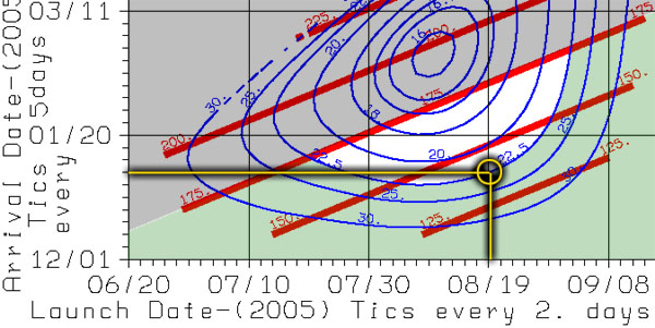
Polaris launches from Terra when Mars is 44.36° ahead. This happens every 26 months
8.6 months later both Polaris and Mars arrives at Point X Terra is now 75.14° ahead of Mars
smAxis = (OrbitRadiuss + OrbitRadiusd) / 2
Now we need to figure the deltaV for Terra-Mars transits.
Hohmann Transfers
Current spacecraft propulsion systems are so feeble that they cannot manage much more than the lowest deltaV missions. So they tend to use a lot of "Hohmann transfer orbits".
A Hohmann orbit between two planets is guaranteed to take the smallest amount of deltaV possible. For the Terra-Mars Hohmann, deltaV is 5,596 m/s.
Notice that the deltaV required to get into orbit is 11,180 m/s while the Terra-Mars deltaV is only 5,596 m/s. As Robert Heinlein noted, once one gets into Earth orbit, you are "halfway to anywhere."
And note that it is not strictly necessary that the destination be a physical planet. It can be a virtual point in space, like a reserved slot in geostationary orbit for your communication satellite obtained at great expense and prolonged negotiation with the International Telecommunication Union. Communication satellites are generally delivered via Hohmann transfer, the equations still work even though there is not a planet at the destination. The virtual point still mathematically moves and acts like a planet, even though there ain't nuttin' there.
Drawbacks of Hohmann Transfers
Unfortunately a Hohmann orbit also takes the maximum amount of transit time. For the Terra-Mars Hohmann mission, transit time is about 8.6 months.
The other drawback is that there are only certain times that one can depart for a given mission, the so-called "Synodic period" or Hohmann launch window. The start and destination planets have to be in the correct positions. For the Terra-Mars Hohmann mission, the Hohmann launch windows occur only every 26 months! If you do not launch at the proper time, when you get to the destination planet's orbit the planet won't be there. And then your life span is the same as your rapidly dwindling oxygen supply.
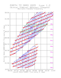
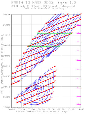
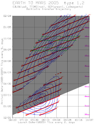
If you are in a hurry and just want the transfer parameters between solar system major planets, you can use Erik Max Francis' Mission Tables. These provide the Hohmann delta-V requirements, the transit time, and the delay between Hohmann launch windows.
If the planets you want are not in the tables (because you've made your own solar system or something), the equations are below:
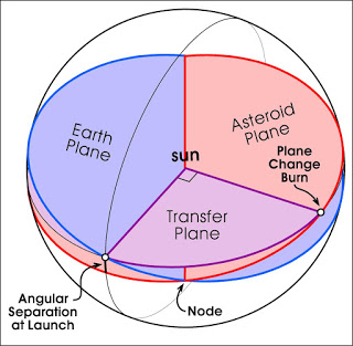
Hohmann Components
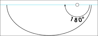
A Hohmann transfer consists of three phases:
Insertion Burn: A large burn to leave circular orbit around starting planet and enter the Hohmann transfer
A long Coasting Phase where the spacecraft travels on an elliptical orbit with engines off
Arrival Burn: A large burn to leave the Hohmann transfer and enter into a circular orbit around the destination planet (otherwise you are doing a flyby mission)
So the total delta V required is the Insertion Burn plus the Arrival Burn.
Note that when launching only an idiot or somebody absolutely desperate will have their Hohmann going contrary to the planet's native orbital motion. Launching in the same direction as the orbital motion means your spacecraft starts out will that motion as free delta V. The Terra-Mars insertion burn requires 32,731 m/s of delta V. Launching with Terra's orbital motion means the ship starts out with 29,785 m/s for free, and only has to burn for an additional 2,946 m/s. And in the same way the Mars arrival burn in theory requires 21,476 m/s but by using Mars orbital velocity the ship only needs 2,650 m/s. The total delta V required is only 5,596 m/s, not the outrageous 54,207 m/s it needs in theory.
Also note that with a Hohmann, the starting point and the ending point will be 180° from each other. That is, if you draw a line from the start point, the center point, and the end point, you will make a straight line.
Calculating Hohmann Delta V
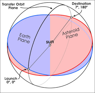
Warning: the following technique is a simplification. It assumes that the planet orbits are perfectly circular, and the two orbits are coplanar. Neither of these are true in reality, but they are close enough for goverment work. The following technique will give you figures that are in the ballpark, but please do not use them for real astrogation. The perfect technique that gives perfect results is a nightmare of mathematical calculation. If you really want to know, find a copy of Fundamentals of Astrodynamics or Introduction to Space Flight and I salute you.
At the start, you have to chose the starting planet and destination planet (or moon, or asteroids, or whatever). Both have to be orbiting the same primary object, the sun or central planet.
First you need "μprimary" ("mu") the gravitational parameter for the sun or planet at the center. If you are calculating Hohmann transfers between planets orbiting Sol, I've precalculated the value of μ for you:
μSolPrimary = 1.32715×10²⁰ m3/s2
If you are doing something fancy like transfers between the moons of Jupiter, you have to calculate μprimary for yourself, using the mass of the central body:
μprimary = 6.674×10⁻¹¹ * Mprimary
where Mprimary = mass of central planet or moon (in kilograms). 6.674×10⁻¹¹ is Newton's gravitational constant expressed in units such that the resulting delta V will be in meters per second, instead of something worthless like furlongs per fortnight. So for Jupiter, Planetary Fact Sheets tell you it has a mass of 1,898.3×1024 kilograms, therefore its μprimary is 1.2669×10¹⁷
For both the starting and destination planets you'll need:
The mean orbital radius in meters, i.e., the distance between the planet and the primary. Remember 1 AU = 1.496×10¹¹ meters, since very few astronomical books are silly enough to give orbital radii in meters.
The planet's mass in kilograms
The planet's mean radius in meters, i.e., distance from the center of the planet and the surface
The altitude of the parking orbit in meters, i.e., the distance between the planet's surface and the orbiting spacecraft. The orbital altitude at the start planet and destination planet can be totally different from each other. To make life easier on you the parking orbits are assumed to be circular.
Now for the Hohmann delta V calculation. This will give the delta V required to leave low orbit around the starting planet and brake into low orbit around the destination planet. For a crewed mission presumably the crew want to return home again, so you'll have to do the calculations over again with the start and destination data swapped. This will give the delta V for the homeward trip. Add these together to find the minimal delta V rating for the spacecraft.
Yes, there certainly are a lot of equations. That's why they call it rocket science. You probably should make a spreadsheet or something to do the work for you. I tried to encode the following into a spreadsheet (download Microsoft Excel 97-2003 XLS, download Libre Office Calc ODS). It may contains mistakes, use at your own risk.
The "s" subscript means "starting planet" and the "d" subscript means "destination planet". Note that this symbol "∞" should be an infinity symbol, a figure 8 lying on its side. Apologies if your browser cannot render it. In some textbooks they use instead the subscript "inf".
ParkingOrbitRadiusd = radius of ship's parking orbit at destination planet (m)
VelocityescD = local escape velocity from destination planet (m/s)
DeltaVd = delta V required for spacecraft to leave Hohmann transfer and enter parking orbit around destination (m/s)
DeltaV = actual total delta V needed for the entire Hohmann transfer, which is what you were doing all these calculations for in the first place
NOMENCLATURE NOTE:
Depending upon which NASA document you are reading, Velocity∞s is also called Departure V-infinity or C3. In missions it is sometimes called Trans-{destination planet}-Injection, e.g.,TMI = Trans-Mars Injection.
Velocity∞d is also called Arrival V-infinity or V∞. In missions it is sometimes called {destination planet}-Orbit Insertion, e.g.,MOI = Mars Orbit Insertion.
Example
For a Terra-Mars Hohmann with central body being Sol, Terra is starting planet, Mars is destination planet.
Mass of Sol = 1.9885×1030 kg = Mprimary
Terra's orbital radius = 1.000 AU = 1.496×10¹¹ meters = OrbitRadiuss
Mars orbital radius = 1.524 AU = 2.280×10¹¹ meters = OrbitRadiusd
Mass of Terra = 5.9720×1024 kg = Ms
Mass of Mars = 6.4171×10²³ kg = Md
Mean Radius of Terra = 6.3710×10⁶ m = PlanetRadiuss
Mean Radius of Mars = 3.3895×10⁶ m = PlanetRadiusd
Terra Parking Orbit Altitude = 300 km = 300,000 m = ParkingOrbitAltitudes
Mars Parking Orbit Altitude = 300 km = 300,000 m = ParkingOrbitAltituded
So the Polaris has to be capable of 5,684 m/s of delta V in order to do the Terra-Mars Hohmann transfer from Low Earth Orbit to Low Mars Orbit.
The Vis Viva Equation
How does the above mess of equations work? By the power of the Vis Viva Equation aka "orbital-energy-invariance law". It is used multiple times.
If you don't give a rat's heinie about how this works, please skip ahead to the next section.
If a planet, moon, spacecraft, or whatever is in an elliptical (non-circular) orbit around a primary object (sun or moon), the Vis Viva equation is:
μprimary = G * Mprimary
V = sqrt[ μprimary * ((2/r) - (1/a)) ]
where
Mprimary = mass of primary object (kg) G = Newton's constant of gravitation = 6.674×10⁻¹¹ N⋅kg-1⋅m2 μprimary = standard gravitational parameter of the primary object V = orbital velocity at a given point along the elliptical orbit (m/s) r = distance from primary of the given point along the elliptical orbit (m) a = semi-major axis of elliptical orbit (m) sqrt[x] = square root of x
According to Kepler's Third Law, a planet in an elliptical orbit around a primary has a different orbital velocity at different points in the orbit. The closer that orbital point is to the primary, the faster the orbital velocity is.
If you have a circular orbit, r = a so the equation reduces to:
V = sqrt[ μprimary / r ]
and the orbital velocity is the same at all points in the circular orbit.
The elliptical Vis Viva equation is used to calculate Velocitys and Velocityd.
The circular Vis Viva equation is used to calculate OrbitalVelocitys, OrbitalVelocityd, ParkingOrbitCircularVels, and ParkingOrbitCircularVeld
SynodicPeriod = 67,359,430 seconds = 26 months = 2.14 years
Calculating Launch Timing
This is for calculating two things:
What is the configuration of the two planets indicating it is time to launch?
If you do a Hohmann from planet A to planet B, how long do you have to wait on planet B before the launch window to planet A opens?
For the first question, the best I can do is indicate the angular separation between the two planets when the Hohmann window opens. For example: with the Terra-Mars Hohmann, when the launch window opens, what is angle Terra-Sol-Mars? Note that 0° is where the start planet is at. And at the end of the Hohmann journey, both the spacecraft and the destination planet will be at 180° from the the location of the start planet at the beginning of the journey.
Since Phase Angle α is positive, Mars is ahead of Terra.
For the Mars-Terra Hohmann, Phase Angle α = -1.31229 radians, or -75.19° behind Mars.
Calculating Stayover Time Before Return Trip
For details about how long the ship will have to delay at Mars before the return trip Hohmann window opens, refer here
HOHMANN WAITING TIME
In a typical round trip, you start at a planet (say, Earth), then execute a Hohmann transfer to another planet (say, Mars). However, you cannot return immediately, since Earth and Mars are then not in the right places. You must wait a certain amount of time before taking another Hohmann transfer back.
How long will that be?
Working out the problem turns out to be relatively straightforward. (For maintaining intuition, I'll continue with the example of visiting Mars, but note that the analysis remains generally applicable.)
First, we define four times:
t0: the time of departure from Earth.
t1: the time of arrival at Mars.
t2: the time of departure from Mars.
t3: the time of arrival at Earth.
Next, we define the (heliocentric) angular position of these planets at given times. As time progresses over the planet's orbital period, these angles sweep out 2π radians of passage over a single planetary year (a period of time PE and PM for Earth and Mars, respectively). We are only interested in their values at the four points above, though. E.g. θM,2 is the angle of Mars at time t2.
We need to define how these angles relate to each other. Let's call tH := t1-t0 the duration of the Hohmann transfer; notice that it is the same going out as coming back. For the time period t0 to t1, the spacecraft is on a Hohmann transfer from Earth to Mars. The angles relate as:
In English, this just says that the (angular) positions of both Earth and Mars advance over the time of the outgoing transfer.
At Mars, we'll wait for some unknown time tW (waiting time). Again, the planets' angular positions advance:
Finally, coming back, we do another Hohmann:
We still need some more information to solve this problem, though. The first two pieces are that a Hohmann transfer always takes you an angle π around the center:
The first equation says that the spacecraft departing Earth must arrive at Mars after going halfway around the orbit, while the second says that the spacecraft leaving Mars must arrive back at Earth, again after a half-orbit. We need to be more-careful, though. Although the angles for the Earth and Mars can be taken to increase monotonically, one of them might do a full orbit while the other has not. We therefore need to be able to add/subtract multiples of 2π of the angles to get them to agree:
We need just one more equation. The entire problem can be shifted by a constant amount around the Sun. To constrain it, without loss of generality we can simply set:
(I'll also rename the remaining k1 to just k.)
We can rewrite this huge mess of equations as a matrix equation to impose some semblance of sanity on the complexity:
Solving this is not too difficult (I did it by hand first before checking my result with sympy). The only part of it we care about is the value for tW, which works out to be:
Because k is just some integer, we can remove that -1. Generalizing the notation a little, so that the home planet has period P0 and the visited planet has period P1, we get:
For k, any value can be chosen so long as the resulting tW is nonnegative.
This was the result I gave here (the Google+ question which nerd-sniped me into doing this whole thing). I'm fairly convinced it's correct, but, it's still a little unsatisfactory. Choosing k from the integers is obnoxious. It would be nice to choose it from the natural numbers (i.e., ℕ := {1,2,3,…}), and thereby get an increasing sequence of possible departure dates, starting from a value that is the earliest.
Requiring that tW≥ 0, some algebra shows that, if P0 > P1, then we must have k ≥ (-2tH)/(P0). Similarly, if P0 < P1, then k ≤ (-2tH)/(P0). And, of course, if P0 = P1, then the planets are co-orbital and you cannot travel between them with Hohmann transfers (so we shall assume this is not the case forthwith).
We now want to generate a sequence of k values from natural-valued n values that produces the correct result either way:
Some ad-hoc finagling with the intersection of these lines in the middle produces:
By substituting back into our answer, we can get an equation that tells you every possible waiting time, starting from the first, indexed by n ∈ ℕ = {1,2,3,…}:
I'm less-confident of this result than the previous but, as we'll see below, it seems to work—at-least for the P0 < P1 case I tested.
Let's check and demonstrate our work by returning to the Earth/Mars example we started with.
The actual values are (note sidereal value for Pi whereas Gregorian calendar used to convert from months):
P0 = 365.256363004 P1 = 686.980 tH =“8.5 months” ≈ 259 days tW =“14.9 months” ≈ 454 days
According to our first formula, we get:
k
tW
-3
≈ 1235 days
-2
≈ 455 days
-1
≈ -325 days
0
≈ -1105 days
1
≈ -1885 days
2
≈ -2665 days
3
≈ -3445 days
Therefore, k must be -2 or less. Notice also the separation between the possible waiting times. They should come in multiples of the transfer window times (because if you miss your departure date for the aligned planets, you'll have to wait until the next transfer window). For Earth/Mars, this is “26 months” ≈ 791 days. Indeed, we see that successive launch times differ by roughly this many days. The agreement is to within 1.5% or so, which is pretty good given the imprecision of tH and the expected tW, as well as the astronomical fact that the orbits are imperfect.
For our second formula, we have:
n
tW
1
≈ 455 days
2
≈ 1235 days
3
≈ 2015 days
This confirms that the formula works when P0 < P1, but the case for P0 > P1 remains untested.
Planetary Transfer Calculator is an on-line calculator for various types of transfers (including Hohmanns and torchship brachistochrone transfers). It can calculate ballistic transfers between planets and moons, and powered (constant acceleration) transfers between stars (including effects of relativity). It can also calculate propagation delay due to the absolute speed of light between planets and moons.
Back-of-the-envelope Orbital Transfer Calculator is an on-line calculator for Hohmann trajectories (only) created by Pete Wildsmith. It is basically a wrapper around Erik Max Francis' BOTE Python library. There are some simplifications which reduce the accuracy a bit, read the docs at the "BOTE Python library" link under "Limitations" for details.
For a more in-depth look at the equations for the deltaV of a given Hohmann mission, go here
There is a more in-depth example of calculating both Hohmann and more energetic orbits using Fundamentals of Astrodynamics at the incomparable Voyage to Arcturus. The entries in question are here,
here, and here.
The discussion is about the superiority of Nuclear-Ion propulsion as compared to Nuclear-Thermal propulsion.
There are good basic tutorials on orbital mechanics and trajectory
here,
here and
here.
Here is an Excel spreadsheet called "Pesky Belter" which will calculate Hohmann deltaV, transit times, and synodic periods.
Erik Max Francis has written a freeware Hohmann orbit calculator in Python, available here. Be warned that the documentation is rudimentary, and operating the calculator requires a beginners knowledge of the Python language.
The Windows utility program Swing-by calculator can be found at http://www.jaqar.com
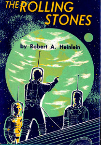
There is a freeware Windows program called Orbiter that allows one to fly around the solar system using real physics. A gentleman named Steven Ouellette has created an Orbiter add-on that re-creates the Rolling Stone from the Heinlein novel of the same name, along with the
mission it flew (follow the above link).
HOHMANN DELTA V INCREASE
In routing a ship to a planet the two chief considerations are
invariably: How much energy will be required and how long
will it take? There are literally millions of paths that will lead
a ship to Mars. Let us see how these two factors aid in the
selection of a route, for some are much easier to follow than
others. SINCE Mars is exterior to the Earth, the projectile or rocket
will have to force its way outward from the Sun—climb uphill so
to speak—in order to get there. This means that at the take-off
it must be moving faster than the Earth, otherwise it will never
be able to make the grade. Now if you were making an urgent
business trip by plane from San Francisco to Chicago, for example, you would hardly continue on to Cleveland or Detroit
and then double back on yourself. Inst so in aiming for Mars
you try not to overshoot the mark but give yourself precisely the
right impetus at the start to reach your destination and no more.
Calculation shows that the minimum velocity required with
respect to the Sun is 19.9 miles per second. (This will vary
slightly depending upon what part of the orbit you attempt to
reach.) The Earth maintains a nearly constant pace in its orbit of
18.5 miles per second. In seeking to reach Mars with as little
expenditure of energy as possible we would be foolish not to
make use of the Earth’s orbital motion which is already ours
for nothing; in fact, we can hardly avoid it. That is, by launching the projectile in the same direction the Earth is headed we
need only give it a speed of 1.4 miles per second in order to
secure the total of 19.9 required. Also, by starting from the
equator at midnight we can pick up an additional 0.3 m.p.s.
from the rotation of the Earth. Thus the shell or spaceship will
depart this world at the comparatively moderate rate of a trifle
over a mile per second—which was very nearly the muzzle
velocity of the Big Bertha that shelled Paris. (We omit from discussion obstacles that arise through atmospheric resistance, force of surface attraction, et cetera, since
such topics would seem to come more properly under the head
of “Piloting” rather than “Astragation.” The figures quoted here
would have to be greatly modified if purely local planetary
problems were included.)
Without going into the technical details in their entirety,
Fig. 12 shows the type of orbit a spaceship would follow in
order to reach Mars by the easiest or so-called 180° route. The
name comes from the fact that departure takes place when the
Earth is on the side of the Sun opposite or 180° from the point
where contact is planned with Mars. Only by shooting off along
a tangent in this way can the ship acquire all of the Earth’s
orbital motion.
TO TAKE the case out of the abstract, suppose that we wished
to arrive at Mars when it was passing the perihelion point of its
orbit on September 17, 1939 at twelve o’clock noon, Central
Standard Time. In order to leave when the Earth is 180° from
this point the passengers must be all aboard on February 24,
1939. All right. It is now February 24, 1939. Here we go! At the start Mars is some one hundred twenty-nine million
miles ahead but the ship rapidly cuts the distance down. By
March 23rd it is reduced to one hundred two million, by April
24th to seventy-four million, and on ]uly 10th they are separated by a mere thirty-nine million miles. And on September
17th as the passengers are preparing to disembark the steward
regretfully announces that they have—missed! By thirty-nine
million miles! The ship made the perihelion point all right but
Mars was forty-two million miles farther east at that moment. This blunder was done purposely to emphasize the obvious
fact which most popular writers for some reason more or less
ignore, that although there is no trouble in calculating exactly
when to leave in order to reach any point on the orbit of Mars
at a set time, this implies no obligation whatever on the part of
the planet Mars to oblige by being there at that time. Before a
ship can be given the green light, the dispatcher must make sure
its orbit properly coincides with the positions of the Earth and
Mars or else it will fail to make connection at the other end of
the line. Thus in the example just cited, although the ship missed
badly by starting on February 24th, investigation shows that
by trying successively later dates it could have gotten onto a
true collision course if departure had been delayed until May
8th. The ship would then have gotten to Mars by January 14,
1940, two hundred fifty-one days later. Astronomical data are
sulficiently precise so that the time of transit could be determined
to within about an hour if necessary, but it is doubtful if schedules will be tabulated closer than about twelve hours since the
last few hundred thousand miles will have to be done by piloting
anyhow. The minimum energy 180° route is the only one generally considered in most popular articles. But if space travel is going to
he limited to a few favorable cases the arrival of a ship from
Mars or Venus will be an occasion for a public demonstration,
as rare as the pack boat from San Francisco to Pago Pago. Somehow this does not fit in with our picture of transportation in
the year 5943 A.D. Recently commentators have begun to speak of the “new
important great circle” airplanes are opening up across the pole
from New York to Chunkiang, Tokyo, and Munnansk. Similarly,
there are other possible paths between worlds besides those
that require the least effort to follow. The bigger the angle between the direction the Earth is moving and the direction the ship takes off for Mars, the more
energy—or what amounts to the same thing—the more money it
is going to take to make the trip. As already explained, this is
because we are using less of the Earth’s motion which is free
and expending more of our own which is apt to be very costly.
But does anyone doubt that the day will come when the value
of an enterprise is reckoned in terms of human necessity rather
than such meaningless symbols as ten million dollars or one
hundred million dollars or one billion dollars? Let us therefore
feel no hesitation about running up a bill on future generations,
payable promptly after the first one thousand years. It can be safely predicted, however, that in terms of whatever
passes for money in 5943, it is going to cost plenty for every day
that is pared off the 180° route to Mars. Suppose now that instead of giving Mars a handicap of 180°, we cut the lead down
to 90°, and successively smaller angles. How much energy will
be needed and how many days will be saved?
Fig. 13 shows the kind of orbit the ship would follow by the
90° route. It is slightly more elongated than the other and
instead of being entirely outside the orbit of the Earth about
forty per cent falls inside. The time of transit is cut down from
two hundred sixty days to one hundred fifty-six days, a saving
of forty per cent. The ship must leave with a speed of 6.2 m.p.s.
relative to the surface and head out an angle of 94° with the
direction the Earth moves. If we assume that the amount of
energy required depends roughly upon the square of the initial
velocity, then Mars via 90° is thirty-two hundred per cent more
expensive than by way of 180°. The reason is perfectly plain.
Before we worked with the Earth in its motion; here we work
nearly at right angles to it. In fact, we have to set a course
which is actually 4° opposite to the Earth’s orbital velocity, or
fire 4° backward, as it were. Note the parallel between a plane taking off a carrier into
the wind and a spaceship leaving the Earth for another planet.
The plane sets a course such that its own speed together with
that of the wind will combine to produce a resultant motion
toward the objective. Similarly, the spaceship takes off at such
an angle that its own speed combined with that of the Earth
puts it into the desired orbit. From this point of view the motion of the Earth may be regarded as a steady wind blowing at
the rate of 18.5 m.p.s. from the west.
NOW let us put the starting point closer and closer to the position of Mars in its orbit. Let us give Mars a handicap of 80°,
70°, 60°—with respect to the Earth. The orbit the ship must follow
is altered drastically as the angle decreases. From a casaba-shaped oval at 90° it collapses through various configurations
resembling watermelons, cucumbers, torpedoes, et cetera, until
at 10° we obtain a narrow cigar-like figure beyond which there
would seem to be little point in pressing matters further. The
journey to Mars by the 10° route takes but eighty-eight days.
Reducing the angle farther does not appreciably reduce the time
beyond a few hours. In fact, as the orbit approaches the limiting figure of a parabola there is an indication that it even increases appreciably. The velocity of the ship with respect to the Sun or the velocity
of the ship in its orbit in the 10° case is not so great as in the
180° and 90° cases; 15.3 m.p.s. as compared with 19.9 and 19.2.
But the velocity of the ship with respect to the Earth is vastly
greater: 21.5 m.p.s. as compared with 1.1 and 6.2. The ship gets
practically no help from the Earth at all, for it must set a course
at an angle of 136° to the Earth’s velocity, or 46° in a direction
opposite to the motion of the Earth. To reach Mars by the 10° route would be for multimillionaires only, for it would be twelve times more expensive than
by 90° and three hundred eighty-two times more than by 180°.
If space travel is to be made available to people of moderate
means as we understand this term now, parity will have to be
fixed at around 0.0001 cent per mile. The longest journey by
way of 180° covers three hundred thirty-eight million miles. At
this rate a round-trip ticket would cost six hundred seventy-six
dollars. But by the 10° route, although the distance is reduced
to fifty million miles, the greater energy needed would boost the
price up to thirty-eight thousand dollars, or two hundred fifteen
dollars per day for mileage alone. These highly eccentric routes could be extremely hazardous
in addition to being highly expensive. For suppose the driving
mechanism failed to work when the time came to land on Mars.
If contact could not be eflected or the passengers and crew
transferred to another ship by rescue squads, they are doomed
to certain destruction. For one of the necessary consequences of
choosing a greatly elongated orbit is that it forces you into the
Sun at perihelion. In the 10° orbit the ship would whip around
the Sun at a distance of two million miles and be speedily converted from a luxurious vehicle for interplanetary travel into a
small comet with a strange spectrum composed of strong metallic lines together with a few faint bands of certain well-known
carbon compounds. It is fun to play with orbits sometimes. Force them to go in
certain directions or make drastic alterations in the elements.
Many of the orbits of newly discovered asteroids and comets
are gradually brought under control by what astronomers have
come to call a “cooking” process; that is, little changes are made
here and there until the best fit possible with the observations
is obtained.
JUST for the devil of it suppose that we take this 10° orbit to
Mars and turn it inside out. Not merely turn it end-for-end but
force the perihelion point to become the aphelion point, and
vice versa. The result is an orbit of exactly the same shape as
before but instead of reaching only as far as Mars now extends
out to nearly three times the distance of Pluto. The period of
an object revolving in this orbit would be three hundred ninety-one years. A path such as a giant interstellar comet might follow—Fig. 15. To travel inward from the Sun—to go from Mars to Earth or
Earth to Venus—means that the ship must fall toward the Sun
or travel more slowly than the planet it leaves behind. To lose
energy might seem comparatively easy in contrast to the effort
of gaining it, but such is not the case, as anyone who has ever
fallen off a train could testify. To reach Venus by the 180° route
the ship must move about 1.6 m.p.s. slower than the Earth. The
ship, therefore, takes off in the opposite direction the Earth is
moving with a speed of 1.6 miles per second. Thus to reach
Venus takes practically the same amount of energy required
for Mars. The journey is considerably shorter, however, only
one hundred forty-six days in all. When taking off from a planet the first consideration must
always be its orbital velocity of revolution. But for a ship cruising far from any large mass it is questionable whether procedure from point to point should invariably be done by orbit with
motors inactive. In many cases it would seem more practicable
to take simply the most nearly direct route possible—the straight
line. Suppose a ship near the orbit of Mars receives orders to meet
a convoy at a distance of one million five hundred thousand miles
within twenty hours. Some energy woudl have to be spent in
getting the ship turned around and headed in the right direction
at the necessary speed. But once under way the motors could
be cut oif and the ship would continue on in a straight line toward the rendezvous position. The only sensible force acting
upon it would be that of the Sun. At the end of twenty hours
the ship would have fallen Sunward by five thousand miles and
be off its course by 0.2°, scarcely enough to be of consequence.
On a long voyage in the vicinity of Venus, however, the effect
of the solar attraction might be more serious. In which case an
occasional blast to Sunward should be suflicient to maintain a
straight-line course.
When a ship begins to enter the outer satellite system, or what
might be called the suburbs of a planet, it will be necessary to
abandon strictly orbital motion and proceed by piloting. The
ship will of course be aware of all satellites in that sector; nevertheless it will be advisable to exercise the greatest caution at
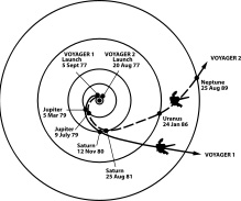
all times. The diagram shows the tangled orbits of the six outer
known satellites of Jupiter (known in 1957. In 2021 the number of known satellites is 79). Once these are safely penetrated
the four large Galilean satellites and the speedy little fifth moon
remain as distinct hazards. Fortunately they revolve in the plane
of the planet’s equator so that practically all risk would be
eliminated by landing in a high altitude. The greatest danger
would be to local traffic moving from one hemisphere to another
—Fig. 16. But as will be shown in this discussion, other considerations make it very doubtful whether Jupiter and Saturn can
ever be successfully colonized. ONE of the favorite devices for introducing the solar system to
the uninitiated is by means of a broad plain on which divers
fruit and vegetables are placed at the proper intervals to represent the Sun and planets. On the scale generally adopted, the Sun is a large pumpkin
or squash. Mercury thirty-six feet away is by tradition a small
pea. Venus and the Earth are larger peas. The Moon nine inches
from the Earth is a radish seed, although some authors favor
mustard seed for the Moon. ]upiter a quarter of a mile away is
an orange. Saturn a smaller orange, and Uranus and Neptune
are plums at distances of a mile and a mile and one-half. Pluto
at two miles from the central pumpkin is still an uncertain quantity, but probably in the pea class with the Earth and Venus. The writer first became aware of this model at about the age
of twelve in one of Sir Robert Ball’s numerous monographs on
astronomy. Since then it has been tuming up regularly in the
popular star books about once or twice a year until now a pronounced allergy has been developed to these fruit-and-vegetable
solar systems. There is something irritating about the smug assurance with which each author goes around depositing oranges
and radish seeds over that two-thousand-acre field. (A ritual
that would certainly cause anyone to be regarded with suspicion of lurking insanity if observed in the act.) You wish
somehow there wasn’t such a finality about the whole performance. That just as the author was laying down the final pea
for Pluto you could grab his arm and cry, “Your neat little solar
system is all wrong! Uranus is closer to the Earth than Mercury
and Pluto is not the farthest planet. Distance is more than merely
a matter of miles!” Anyone making such a ridiculous statement would undoubtedly be considered as of unsound mind himself, an intelligence
unhinged possibly by the reading of too much science-fiction.
Either that or else a visitor from the future to whom the remark
that Pluto is the third nearest planet from the Earth would
sound like the most natural thing in the world. When we say that the town of A is twenty miles away and B
is five miles, therefore B is closer than A, we may be telling the
biggest kind of a falsehood. The trouble is we have told only
a part of the truth—the geometrical part. If the State has built a
beautiful high-gear road to A while the taxpayers on the way
to B have been neglected in this respect, then to all intents and
purposes A is closer than B. Or perhaps the five miles to B goes
through heavy traflic while A is relatively shunned by motorists.
There is a convenient term which we might borrow from optics which is applicable here. This is the notion of “effective distance.” If one beam of light goes through a dense flint prism
and another through an equal length of air, the former is said
to have the longer effective path. Once we begin to take account
of obstacles to be overcome or the energy needed to get from
place to place our whole scale of measurement calls for immediate revision. Space engineers wrestling with the manifold problems of
routing vessels throughout the solar system are going to be
greatly concerned with energy changes or effective distances and
comparatively little with linear changes or geometrical distances.
In going from Planet P to Planet Q there are two fundamental
factors to be considered: (1) the distance made good toward
or away from the Sun; and (2), the relative mass and radius
of the planets involved. These factors may combine in all sorts
of ways that often lead to energy jumps as surprising as those of
the Bohr atom in its heyday. But whereas the Bohr atom led a
carefree existence, emitting and absorbing energy at will, a
spaceship must reckon continually upon the course of future
events. In order to see clearly how the ship’s passage is aifected by
the energy conditions encountered, it is first necessary to get a
picture of the solar system that is utterly different from any
you have ever seen before. But remember that regardless of
how weird it may look, it is just as true a representation in its
way as the old pumpkin-radish-seed model. Fig. 17.
IMAGINE yourself to be an ant crawling over the outside surface of a vast trumpet-shaped structure one thousand feet tall.
It stands upon its small end in an upright position—a highly
unstable state of equilibrium. There is no danger of it toppling
over or collapsing, however. It is only one foot wide at the base
and extends upward Without widening perceptibly almost to
the very top. Then from nine hundred eighty-seven feet to one
thousand feet it suddenly flares out all around like the stem of
a champagne glass to a distance of forty-three hundred feet. This trumpet-shaped structure is an Energy-Distance model of
the solar system. It is not quite so easy to visualize as the one of
flat concentric rings, but then there is no really valid reason
why we cannot represent our solar system by an old-fashioned
phonograph horn as well as a machine-gun sight. We must imagine also that we are constrained to move over the outside surface
of this structure. This means that we are keeping within the
plane of the solar system; we cannot drop above or below the
plane in which the planets circulate. The Sun is supposed to be located at the narrow foot of the
model. Its width of one foot represents the diameter of the Sun
on the scale we have chosen. Now consider the case of an ant
near the Sun who wishes to move away from it; to move outward in space keeping Within the plane of the solar system.
Since he is restricted to the surface his only means of doing
this is by climbing up the long, steep neck of the figure. Thus to
go a very short distance horizontally the ant must do a tremendous
lot of hard Work climbing vertically. Eventually at the nine-hundred-eighty-seven-foot level he comes to line drawn around
the surface which bears an inscription. Slowly he spells it out
letter by letter—ORBIT OF THE PLANET MERCURY. That is, the
distance from the Sun to its first member when measured in
terms of the energy needed to make the pull constitutes ninety-eight point seven per cent of the whole system. Feeling somewhat encouraged, the ant crawls up another six
feet and finds a second line marked ORBIT OF THE PLANET VENUS.
Two feet more brings it to the orbit of the Earth. The going
is much easier now, for the surface is spreading rapidly outward
so that to go from one orbit to another requires hardly any work
at all. From Jupiter clear on out to the rim which marks the
orbit of Pluto is a climb of but eleven inches. Millions of ants for countless millions of years might crawl
around over such a surface, notice vaguely that it was a lot
harder to move over some portions than others, but feel no compulsion to investigate the matter farther. Until one day a certain
ant would analyze the situation very minutely and as a result
would announce that the intensity of the force varied inversely
as the square of the distance from the central vertical axis. This
explained immediately why the force was so strong at the
lower end where the figure was the slimmest and why it was
scarcely perceptible at the upper flared end. Later another ant
developed a theory in which the force was ascribed to the
curvature of the space itself rather than an inherent property
of the matter at the bottom of it. ON THIS MODEL the orbits of the planets would be nearly
circular rings around the extreme top portion, although the orbit
of Mercury would dip slightly at one end. That is because most
of the orbits are almost perfect circles and experience little
change in energy from perihelion to aphelion, except for Mercury which is much more eccentric. The effect would be greatly
exaggerated for a comet. At aphelion the orbit would be nearly
circular like a planet’s. As the comet nears the Sun its path
would begin to drop sharply until the lowest point would be
reached at perihelion. Then the comet would zoom up the other
side of the column tracing out a path identical with the one going downward in reverse. A comet with an orbit approaching
the parabolic like Halley’s would go into a nose dive straight
down the long stem and seem on the verge of shooting off the
bottom. Then it would suddenly perk back and fly upward at
a slowly decreasing pace, leisurely swing around the top rim
and almost—but not quite—make connection with its previous
path. The mass of a comet is so small that it may be disregarded
entirely, reducing it to the same social level as the geometrical
point, or mere locus in space. A planet, however, has an appreciable mass compared with the Sun, and their case is not so
easily set aside. It is hard to represent a planet on our model
because they are in the nature of discontinuities in the smooth
uniformity of the force field. The only reason why you must
take a planet into account at all is because you can get so infernally close to them; right onto their surfaces, in fact. Now the
force of surface attraction depends directly upon the mass of
a planet—that is why Jupiter pulls so hard—and inversely upon
its radius—which is why the tiny white dwarf stars have such
incredible strength. Thus even a small planet at its surface can
attract much more powerfully than the Sun at a distance of a
few million miles. A timely analogy would be that of the lonely
soldier pondering how best to spend his week-end leave. He
is stirred by thought of the potent attractions of the big city far
away, but decides in favor of the small town within easy thumbing distance of camp. Although the Sun maintains the space around it in a state
of tension that ranges from a steep gradient within the orbit of
Mercury out to where it begins to level off beyond Jupiter, there
are pockets within it—the planets—where local conditions are
sharply reversed. On the Energy-Distance model a planet would
appear as a sharp projection or knob depending upon its mass.
Jupiter would be a long icicle hanging down almost to the orbit
of Mercury. Saturn, Neptune and Uranus would be shorter
icicles or stalactites. The Earth, Mars and Venus would be little
more than pin points. The captain of a spaceship approaching Jupiter would not
begin to experience his attraction until within about a million
miles or so of the surface. If for some reason he were unaware
of the planet’s presence, he would be amazed to find his instruments recording an abrupt reversal in gravitational intensity
calculated for that region. He would undergo all the sensations
of a man confidently strolling up the side of a hill who was
unceremoniously precipitated into a hole in the ground. The work required to leave the surface of Jupiter is sufficient
to take a ship from the orbit of Mercury to the orbit of Mars.
Conversely, a ship that lands on Jupiter would have an equal
quantity of work done upon it. (Here we again omit all discussion of practical landing operations.) If space travel can be done
on the principle of the storage batery, so that when going downhill or in the direction of increasing gravitational attraction
energy can be accumulated, a ship arriving upon jupiter will be
fairly bulging with power. But it does not represent any real
gain because it will have to be used up again when the time
homes to leave. It is like entering a country with a favorable rate
of exchange. You are way ahead so long as you stay there, but
your wallet flattens out as soon as you cross the border. THE HUGE MASS of major planets makes it very doubtful
whether they can ever be successfully colonized by beings like
ourselves. Unless a cheap source of energy becomes available
beyond any we can imagine at present—which may easily be the
case—these mammoth hulks seem destined to be shunned forever
owing to their inordinate tenaciousness. Woe to the skipper who
allows his craft to drift within the hold of Jupiter! To approach
and disembark is theoretically quite effortless; all done at Jove’s
personal expense, in fact. But the traveler soon finds to his dismay that he is fast within a gravitational prison from which
escape is possible only by paying an exorbitant ransom. It is one
of those easy-to-get-into, hard-to-get-out-of propositions, like
promising to make a speech or meet a payment months in
advance. This must not be taken to signify that space travel is going to
be limited by the orbit of Mars. Jupiter, Saturn, and Neptune
all have satellites as large as the Moon or Mercury within moderate energy distances. For the inverse square part of Newton's
law works both ways; it makes the force-field build up rapidly
near a body and also peter out rapidly a few diameters away.
Ideal landing fields will undoubtedly be found on Jup III and
Jup IV, which according to the latest estimates are a trifle larger
than Mercury and so far from Jupiter that his attraction would
be a minor consideration. Saturn, Neptune, and Uranus are curious examples of massive
bodies with feeble surface attractions. They are emasculated, so
to speak, because they are unable to make effective use of the
matter with which they are endowed. A planet behaves much
as if it were a ballbearing surrounded by a film of soap bubble.
It attracts at the surface as if its mass were all concentrated at
the center. Saturn has eighty-three per cent of Jupiter’s girth but
only thirty-three percent of his mass. Result is that Saturn attracts
on the surface scarcely more than Earth. But shrink Saturn
down by twelve thousand miles—get twelve thousand miles
closer to him—and his surface gravity will promptly equal that
of Jupiter’s. It produces a queer feeling to think that we could walk around
over Saturn with little more exertion than on the Earth. Yet
Saturn is one of the most powerful disturbing objects in the
solar system affecting the motions of Neptune and Jupiter while
the Earth can barely produce a tremor as close as Mars or Venus.
Which is one for you to figure out. Our planet is rather exceptional in that its surface gravity is
fairly large, perhaps unduly so compared to the muscular development of its inhabitants. The dinosaurs, for example, were
forced out of the race entirely because their size and strength
were so out of proportion to their weight. Which might cause
one with a bent for ecology to toy with the idea that maybe we
are not natives of the Earth at all but creatures originally spawned
from some other world of lesser gravitational power. In short,
that we need not continue wondering what the Martians are like
because we are the descendants of pre-historic Martian invaders!
Leaving such highly speculative material for other writers
in science fiction, it may well be questioned whether the
energy difference in a transition from planet to planet is the
factor of main importance. There can be no argument that going
uphill from an inner orbit to an outer orbit energy will have to
be expended in the climb. But when work is being done on a
ship as in the drop-down to an inner orbit or surface of a planet,
energy will still have to be used in order to cushion the fall.
Otherwise a ship would arrive on Jupiter at the rate of around
one hundred forty thousand miles an hour. An engineer planning a trip, therefore, would probably make
a more accurate estimate if he takes into account the total energy
involved regardless of which way it is acting. This is plain common sense and agrees with our everyday experience. Thus any
astronomer at Mount Wilson can testify that the strain on the
leg muscles is the same whether they are used in pulling yourself up the twenty miles to the Observatory, or in bracing yourself on the way down. On the basis of the total needed to reach a planet’s surface
from the Earth—energy from orbit-to-orbit and from surface-to-surface—the solar system presents such a scrambled appearance
that the familiar old astronomer with his fruit and vegetables
would never recognize it in a lifetime. Here are the distances to
the various members in terms of the distance to Venus, which
maintains its position as our nearest neighbor:
EFFECTIVE OR ENERGY DISTANCES TO THE PLANETS
1. EARTH TO VENUS
1.00
2. EARTH TO MARS
1.02
3. EARTH TO PLUTO
2.50
4. EARTH TO URANUS
2.91
5. EARTH TO NEPTUNE
3.91
6. EARTH TO SATURN
4.00
7. EARTH TO MERCURY
4.19
8. EARTH TO JUPITER
7.11
9. EARTH TO SUN
543
Thus by taking what the mathematician would call the absolute sum of the energy distances to the planets, Pluto becomes a
comparatively close object while Mercury is removed to the
border of the system. Notice also that the planets fall into rather
distinct groups: (1), Venus and Mars; (2), Pluto, Uranus, and
Neptune; (3), Saturn and Mercury; (4), Jupiter and his satellite
system. Other solar systems might be devised even more outlandish
than the Energy-Distance Model, yet be just as true a representation as one can readily visualize. Come to think of it, an
astronomer’s life is devoted chiefly to sifting illusion from reality.
Trying to find where things really belong in this universe. Mars
may be forty million miles away but springtime on the Syrtis
Major isn’t very much longer than ours.
Terra Space Station and the school ship Randolph are in a circular orbit 22,300 miles above the surface of the Earth, where they circle the Earth in exactly twenty-four hours, the natural period of a body at that distance.
Since the Earth's rotation exactly matches their period, they face always one side of the Earth — the ninetieth western meridian, to be exact. Their orbit lies in the ecliptic, the plane of the Earth's orbit around the Sun, rather than in the plane of the Earth's equator. This results in them swinging north and south each day as seen from the earth. When it is noon in the Middle West, Terra Station and the Randolph lie over the Gulf of Mexico; at midnight they lie over the South Pacific.
The state of Colorado moves eastward about 830 miles per hour. Terra Station and the Randolph also move eastward nearly 7000 miles per hour — 1.93 miles per second, to be finicky. The pilot of the Bolivar had to arrive at the Randolph precisely matched in course and speed. To do this he must break his ship away from our heavy planet, throw her into an elliptical orbit just tangent to the circular orbit of the Randolph and with that tangency so exactly placed that, when he matched speeds, the two ships would lie relatively motionless although plunging ahead at two miles per second. This last maneuver was no easy matter like jockeying a copter over a landing platform, as the two speeds, unadjusted, would differ by 3000 miles an hour.
Getting the Bolivar from Colorado to the Randolph, and all other problems of journeying between the planets, are subject to precise and elegant mathematical solution under four laws formulated by the saintly, absent-minded Sir Isaac Newton nearly four centuries earlier than this flight of the Bolivar — the three Laws of Motion and the Law of Gravitation. These laws are simple; their application in space to get from where you are to where you want to be, at the correct time with the correct course and speed, is a nightmare of complicated, fussy computation.
From SPACE CADET by Robert Heinlein (1948)
Rocket Railroad
You are probably using Hohmann transfer orbits because your rocket ain't a torchship. That is the spacecraft has such a pathetically small amount of delta-V that it is forced to use bargain-basement bin cheap Hohmanns instead of fast but hideously expensive Brachistochrone tranfers.
Since the ship is on such a tight delta-V budget it cannot afford to leave the pre-plotted Hohmann trajectory. If you do, you'll run out of the propellant you need to reach your destination, the ship will sail off into the Big Dark, and everybody will die when the oxygen runs out. This was highlighted in a famous story called The Cold Equations by Tom Godwin.
The net result is that when it comes to side trips, rockets are about as capable of that as is a railroad locomotive. The rocket has to stick to its planned Hohmann like it was a choo-choo train on solid steel girders. Much like a locomotive, leaving the tracks for an off-road excursion is a disaster (yes I know that some cargo spacecraft are arranged like train with the engines in the front dragging the cargo behind, but that's another matter).
RUNNING ON RAILS
In spite of the title this post is about spaceships, not trains. It is inspired by commenter Ferrell's remark, in discussion of the aesthetics of space travel, that 'cycler stations' seem more like railroads than ships. To expand on my own response there, this is largely true of spacecraft in general, at least those without magitech drives.
Trains, it has been observed, differ from other common terrestrial vehicles in that they have no steering wheel. Once they leave the station platform they go not where 'the governor [helmsman] listeth,' but where the tracks take them. Spaceships may have a joystick for attitude control, but once they light up their main drive they go where the laws of physics take them. As I noted last year in Space Warfare IV: Mobility, the way they actually get around resembles
... self-propelled artillery shells. Once they fire themselves into a particular orbit they can change that orbit only by another burst of power, expending more propellant in the process.
Regular readers here are probably geeky enough that you already know this, and in particular you likely appreciate the tactical military implications — what space wargamers call vector movement, AKA why spaceships don't maneuver the way Hollywood usually portrays. So why am I beating you over the head with it? Because it is so easy to forget that this applies not only to tactical maneuvers but to strategic or 'operational' movements, and to commercial traffic.
If a spaceship in Earth orbit is fueled up and ready to go to Mars, once you punch the 'go' button you are on your way to Mars. Yes, in the early stages of your departure burn you can abort back to Earth orbit (or, very occasionally, to lunar orbit). But once past that initial abort window any subsequent change of orbit will, in nearly all cases, take you only on a long, slow trip to nowhere.
This applies most rigidly to economical Hohmann (or near-Hohmann) transfer orbits, but it applies with nearly as much force even to fast ships taking steep orbits. Unless provided for in your mission plan, the chances that your fuel allowance permits you to change orbit to one that will get you somewhere else is slim to none.
Military missions may — and certainly should, if possible — provide an abort option that will get you to some friendly base before life support runs out. Commercial missions, probably not: These trips will be costly enough without carrying along extra fuel and life support for a change of destination. And for most space emergencies such an abort would be useless anyway — whatever keeps you from safely reaching Mars would make it even harder to reach anywhere else.
Thus space operations will 'run on rails,' with the route and destination fixed not just by the space line's policy but by constraints of time, motion, and propellant supply.
All of which has some interesting secondary implications, ranging from space rescue to command structure. Rescue is plausible between ships on similar orbits, as in Heinlein's Rolling Stones, where Dr. Stone transfers to a nearby liner, black bag in hand, to fight a disease outbreak on board. But if two ships are passing on different orbits, don't expect one to be able to assist the other. Similarly, 'lifeboats' are pretty much useless in deep space — if you take to the boats you're still on the same orbit as the stricken ship, and unless the lifeboats have delta v and life support comparable to the ship itself they won't help. (Two hab structures with independent life support are a much better bet.)
The constraints of space motion also raise a question about who should be in command. In the movie Casablanca, Rick Blaine suggests to Ilsa that they get married on a train. "The captain of a ship can perform marriages; why not the engineer on a train?" But the 'captain' of a train is not the engineer; it is the conductor. (In British railway usage, not the driver but the guard.)
At sea and in the air a pilot/navigator traditionally has command, because they are the most skilled at handling the vehicle under abnormal conditions, to change course and reach sheltered waters or a safe landing. But in space, especially deep space, brilliant shiphandling is probably not an option. Survival, if possible, will generally depend on the crew's ability to function as a social unit, and on the life support system holding out. In human dramatic terms a spaceship is more like an isolated outpost than any terrestrial vehicle.
Finally, a way that spaceships differ even from trains is that nearly all travel is nonstop, from point of origin to final destination. Terrestrial vehicles can and often do make intermediate stops along the way, each time letting off some passengers and cargo, and taking on others. This trip pattern lends itself well to RPGs, picaresque scenarios in general, and especially episodic television, with each waypoint an Adventure Town.
This is practical because ships and trains (or caravans, etc.) lose little time and expend insignificant fuel in making intermediate stops. Planes need extra fuel to climb back to cruise altitude, but they can top off their tanks, and by not carrying fuel for a nonstop trip they can usually carry more payload.
Alas, it does not work that way in space. Spaceships don't burn their fuel while cruising; they burn it to speed up and slow down. So even if several planets were neatly lined up, each intermediate stop would involve major burns. Carrying passengers or cargo to Saturn, with intermediate stops at Mars and Jupiter, means accelerating and decelerating your Saturn-bound manifest three times — a much better way to reach the poorhouse than Saturn. Ships may make several passages before returning to their home base, but nearly all passengers and cargo will turn over at each port of call. (Cargo may not travel by 'ship' at all.)
There are some specialized exceptions to most or all of these rules. And, of course, with a suitable magitech drive all bets are off. But that is a topic for a different discussion.
THE LINER Pegasus, with three hundred passengers arid a crew of sixty, was only four days out from Earth when the war began and ended. For some hours there had been a great confusion and alarm on board, as the radio messages from Earth and Federation were intercepted. Captain Halstead had been forced to take firm measures with some of the passengers, who wished to turn back rather than go on to Mars and an uncertain future as prisoners of war. It was not easy to blame them; Earth was still so close that it was a beautiful silver crescent, with the Moon a fainter and smaller echo beside it. Even from here, more than a million kilometers away, the energies that had just flamed across the face of the Moon had been clearly visible, and had done little to restore the morale of the passengers.
They could not understand that the law of celestial mechanics admit of no appeal. The Pegasus was barely clear of Earth, and still weeks from her intended goal. But she had reached her orbiting speed, and had launched herself like a giant projectile on the path that would lead inevitably to Mars, under the guidance of the sun's all-pervading gravity. There could be no turning back: that would be a maneuver involving an impossible amount of propellant. The Pegasus carried enough dust in her tanks to match velocity with Mars at the end of her orbit, and to allow for reasonable course corrections en route. Her nuclear reactors could provide energy for a dozen voyages—but sheer energy was useless if there was no propellant mass to eject(and if you say "but what about reactionless thrusters?" RocketCat will give you an atomic wedgie). Whether she wanted to or not, the Pegasus was headed for Mars with the inevitability of a runaway streetcar. Captain Halstead did not anticipate a pleasant trip.
The words MAYDAY, MAYDAY came crashing out of the radio and banished all other preoccupations of the Pegasus and her crew. For three hundred years, in air and sea and space, these words had alerted rescue organizations, had made captains change their course and race to the aid of stricken comrades. But there was so little that the commander of a spaceship could do; in the whole history of astronautics, there have been only three cases of a successful rescue operation in space.
There are two main reasons for this, only one of which is widely advertised by the shipping lines. Any serious disaster in space is extremely rare; almost all accidents occur during planetfall or departure. Once a ship has reached space, and has swung into the orbit that will lead it effortlessly to its destination, it is safe from all hazards except internal, mechanical troubles. Such troubles occur more often than the passengers ever know, but are usually trivial and are quietly dealt with by the crew. All spaceships, by law, are built in several independent sections, any one of which can serve as a refuge in an emergency. So the worst that ever happens is that some uncomfortable hours are spent by all while an irate captain breathes heavily down the neck of his engineering officer.
The second reason why space rescues are so rare is that they are almost impossible, from the nature of things. Spaceships travel at enormous velocities on exactly calculated paths, which do not permit of major alterations—as the passengers of the Pegasus were now beginning to appreciate. The orbit any ship follows from one planet to another is unique; no other vessel will ever follow the same path again, among the changing patterns of the planets. There are no "shipping lanes" in space and it is rare indeed for one ship to pass within a million kilometers of another. Even when this does happen, the difference of speed is almost always so great that contact is impossible.
Holden leaned back in his chair and listened to the creaks of the Canterbury's final maneuvers, the steel and ceramics as loud and ominous as the wood planks of a sailing ship. Or an Earther's joints after high g. For a moment, Holden felt sympathy for the ship.
They weren't really stopping, of course. Nothing in space ever actually stopped; it only came into a matching orbit with some other object. They were now following CA-2216862 on its merry millennium-long trip around the sun.
From LEVIATHAN WAKES by "James S.A. Corey" (2011). First novel of The Expanse
Mid-Course corrections
When a probe or spacecraft performs a maneuver, the idea is to enter into a pre-calculated trajectory (hopefully arriving at your destination). But nobody and nothing is perfect. The performance of the maneuver might be a hair off, though not enough to be immediately noticeable. Mission Control or the spacecraft's astrogator has the job of monitoring the spacecraft's current position and vector at this specific point in time, to see if the spacecraft is still on track for the specified trajectory. If it is not in the groove, the astrogator will calculate a mid-course corrections (Trajectory Correction Maneuver or TCM). This is a tiny maneuver to put the spacecraft back on track.
Currently I have no idea how to calculate such a thing. In Proceeding of the Symposium on Manned Planetary Missions 1963/1964 they suggested that with then-current navigation gear the delta V required for TCM on the Terra-Mars trajectory was about 105 m/s and 92 m/s for the Mars-Terra trajectory.
Other Transfer Orbits
CONJUNCTION CLASS artwork by Edward Bell
CONJUNCTION CLASS
For high-thrust rockets, the most fuel-efficient way to get to
Mars is called a Hohmann transfer. It is an ellipse that just
grazes the orbits of both Earth and Mars, thereby making the
most use of the planets’ own orbital motion. The spacecraft
blasts off when Mars is ahead of Earth by an
angle of about 45 degrees (which happens every
26 months). It glides outward and catches up
with Mars on exactly the opposite side of
the sun from Earth’s original position. Such
a planetary configuration is known to astronomers
as a conjunction. To return, the
astronauts wait until Mars is about 75 degrees
ahead of Earth, launch onto an inward
arc and let Earth catch up with them.
Each leg requires two bursts of acceleration.
From Earth’s surface, a velocity boost of
about 11.5 kilometers per second breaks free of
the planet’s pull and enters the transfer orbit. Alternatively,
starting from low Earth orbit, where the
ship is already moving rapidly, the engines must impart about
3.5 kilometers per second. (From lunar orbit the impulse would
be even smaller, which is one reason that the moon featured in
earlier mission plans. But most current proposals skip it as an
unnecessary and costly detour.) At Mars, retrorockets or aerobraking
must slow the ship by about 2 kilometers per
second to enter orbit or 5.5 kilometers per second
to land. The return leg reverses the sequence.
The whole trip typically takes just over two
and a half years: 260 days for each leg (increasing astronaut exposure to galactic cosmic radiation) and
460 days on Mars. In practice, because the
planetary orbits are elliptical and inclined,
the optimal trajectory can be somewhat
shorter or longer. Leading plans, such as
Mars Direct and NASA’s reference mission,
favor conjunction-class missions but quicken
the journey by burning modest amounts
of extra fuel. Careful planning can also ensure
that the ship will circle back to Earth naturally
if the engines fail (a strategy similar to that
used by Apollo 13).
OPPOSITION CLASS artwork by Edward Bell
OPPOSITION CLASS
To keep the trip short (reducing astronaut exposure to galactic cosmic radiation), NASA planners traditionally considered opposition-class trajectories,
so called because Earth makes its closest approach to Mars—a configuration
known to astronomers as an opposition—at some point in the mission choreography.
These trajectories involve an extra burst of acceleration, administered en route. A typical
trip takes one and a half years: 220 days getting there, 30 days on Mars and 290 days coming
back. The return swoops toward the sun, perhaps swinging by Venus, and approaches
Earth from behind. The sequence can be flipped so that the outbound leg is the longer one.
Although such trajectories have fallen into disfavor—it seems a long trip for such a short
stay—they could be adapted for ultrapowerful nuclear rockets or “cycler” schemes in
which the ship shuttles back and forth between the planets without stopping.
LOW THRUST artwork by Edward Bell
LOW THRUST
Low-thrust rockets such as ion drive save fuel but are too
weak to pull free of Earth’s gravity in one go (high specfic impulse but very low thrust). They must
slowly expand their orbits, spiraling outward like a car switchbacking
up a mountain. Reaching escape velocity could take up
to a year, which is a long time to expose the crew to the Van
Allen radiation belts that surround Earth.
One idea is to use low-thrust rockets
only for hauling freight. Another is to
move a vacant ship to the point of escape,
ferry astronauts up on a “space
taxi” akin to the shuttle and then fire another
rocket for the final push to Mars.
The second rocket could either be high or
low thrust. In one analysis of the latter
possibility, a pulsed inductive thruster
fires for 40 days, coasts for 85 days and
fires for another 20 days or so on arrival
at the Red Planet.
A VASIMR engine opens up other options.
Staying in low gear (moderate
thrust but low efficiency), it can spiral
low efficiency), it can spiral
out of Earth orbit in 30 days. Spare propellant shields the astronauts
from radiation. The interplanetary cruise takes another 85
days. For the first half, the rocket upshifts; at the midpoint it begins
to brake by downshifting. On arrival at Mars, part of the
ship detaches and lands while the rest—including the module for
the return flight—flies past the planet, continues braking and enters
orbit 131 days later.
From HOW TO GO TO MARS by George Musser and Mark Alpert (Scientific American March 2000)
INTERPLANETARY TRAJECTORIES
Update 11-24-19: revised delta-vees for Phobos trip, appended below
The planning of interplanetary flights, such as from Earth to Mars, uses basic orbital mechanics. As long as the spacecraft speed does not reach solar escape speed, the form of the orbital trajectory about the sun will be an ellipse. There are “min energy” trajectories, and there are faster trajectories, but all these trajectories will be ellipses.
The basics of elliptical orbits are given in Figure 1, including just about all the relevant
analysis equations, plus a little more. An ellipse is a symmetrical closed curve
containing two foci. The central body
occupies one focus, the other is
unoccupied. These foci are located
farther from the center in the more eccentric ellipse. A circular orbit is a sort of “degenerate”
ellipse with zero eccentricity, so that
the foci come together at the center. I
wrote this for a diverse audience of both technical and non-technical people.
Bear in mind that these analytical solutions apply only
to a 2-body problem (one object orbiting a central body). The 3-body problem (object and two bodies)
requires integration of the equations of motion for an exact solution.
Figure 1 – Basics of Elliptical Orbits (2-Body Problem) click for larger image
For interplanetary trips,
we are talking about trajectories where the central body is the
sun. However, this same analysis applies to orbits about
the Earth or any other body. The key
features of elliptical orbits are the speeds,
which vary around the path, and
the min and max distances from the central body.
“Perihelion” is the end apex of the ellipse closest to the sun, where the speeds are highest. “Aphelion” is the end apex of the ellipse
farthest from the sun, where speeds are
lowest. The corresponding terms for an
orbit about the Earth are “perigee” and “apogee”. For the moon, they are “pericynthion” and
“apocynthion”. Thus the
abbreviation “per” applies to the closest approach, and “apo” the farthest approach, regardless of the central body.
When looking up tables of characteristics of astronomical
bodies, the description of their orbits
is usually cast as min and max distances from the central body. Those would be rper and rapo, respectively. Their average is the semi-major axis length
“a”. The eccentricity “e” and the period
“P” are easily computed from these distances,
all as given in Figure 1.
Further, the distance of the foci
from the center of the ellipse “c”, and
the length of the semi-minor axis “b”,
are also easily computed, and
given in the figure, as is the equation
for x-y coordinates all along the ellipse,
where these x-y coordinate are centered at the center of the ellipse.
The equation giving velocity at any radius “r” from the
central body is actually quite simple, as
shown in the figure above. Note
that “r” is bounded: rper
< r < rapo. There is no
simple equation giving time at any particular point around the elliptical
path. Centuries ago, it was
said “equal areas are swept out by the radius vector from the central
body in equal amounts of time”.
Today, we would say
that the time along a segment is proportional to the area swept out by the
radius vector from the central body to the object, moving along that segment. You can obtain that time by integrating the
area under the segment from one point to another, and adding or subtracting the appropriate
triangle area. All of this should be
evident upon inspection of Figure 1 above, particularly noting the shaded area.
The “extras” in Figure 1 are the equations for
calculating the escape velocity and low circular orbit velocity of any
celestial body, plus a form of
mechanical energy conservation as you approach (or depart from) a body in an
unpropelled state.
Hohmann Min-Energy Transfer
These trajectories are the ones with the minimum velocity
requirements for travel. The perihelion
of the transfer ellipse is located at the orbit of the Earth on one side of the
sun. The apohelion of the transfer
ellipse is located at the orbit of Mars on the other side of the sun. See Figure 2. Because the orbit of Earth is slightly
elliptical, and Mars more so, these distances vary somewhat. Using the average values gets you into the
ballpark, but you should really use the
worst case to size your spacecraft’s propulsion capability!
Note that because the Hohmann transfer ellipse is tangent to
a very-nearly-circular planetary orbit at each end, then the planetary velocity and transfer
orbit velocity vectors are essentially parallel at each end. What is ordinarily a vector subtraction
devolves to a simple scalar subtraction,
for determining the velocities with respect to the planet, at each end.
That is only true when the perihelion or the apohelion of the
orbit are located at the appropriate planetary orbit distance from the sun.
Specifically, the
velocity vector of the spacecraft with respect to the planet is the velocity vector
of the spacecraft with respect to the sun,
minus the velocity vector of the planet with respect to the sun:
spacecraft
Vwrt planet = Vwrt sun – Vplanet wrt sun where V is a vector velocity
Figure 2 – The Hohmann Min-Energy Transfer Ellipse Earth-to-Mars and Back click for larger image
An Approximation to the 3-Body Problem
The trouble the above evaluations right at perihelion and
apohelion is that these are 2-body (spacecraft and sun) analyses, and the close-vicinity dynamics of departure
and arrival are fundamentally a 3-body problem (spacecraft-sun-planet). As already stated, it takes computerized 3-body analysis to get
velocity requirements and detailed localized trajectories exactly right. Yet,
you can get very, very close to
the velocity requirements with the following approximation technique.
As in the above discussion,
you do the vector velocity subtraction to find the velocity of the
spacecraft with respect to the planet,
at the perihelion and apohelion conditions. For only Hohmann min energy transfer, this calculation devolves to a simple scalar
subtraction, because the vectors are
parallel. Either way, there is a velocity magnitude involved.
The approximation is to treat this relative velocity
with respect to the planet as a velocity “very far from the planet”, and to approximate the pull of the planet’s
gravity during the close encounter as an unpowered gravitational acceleration
toward the planet, from “very far” to
“very close”. This is done with conservation
of mechanical energy, based on the
“far from planet” velocity magnitude (with respect to the planet), which makes the vector direction more-or-less
irrelevant, except to the trajectory
details. Conservation of mechanical
energy says:
0.5 m Vfar2
= 0.5 m Vnear2 - change-in-PE far-to-near, where m = spacecraft mass
This approximation then makes use of the very convenient
fact that the change in potential energy from very far to very near is, in point of fact, numerically equal to the spacecraft kinetic
energy associated with the escape velocity of the planet:
0.5 m Vesc2
= change-in-PE far-to-near
Thus, after dividing
off the “0.5 m” factors common to all three terms, we have a very simple way to estimate the
spacecraft velocity magnitude with respect to the planet, once it is “very close”. This velocity would apply for either entry
into planetary orbit, or for the initial
direct entry into the local atmosphere for aerobraking (of any type). That simple equation is:
Doing the full 3-body problem on the computer refines the actual
trajectory to be flown, but does not
refine the spacecraft propulsion velocity requirements very much at all, beyond these simple estimates. These estimates are really quite good, and apply to departure as well as arrival.
This is illustrated in Figure 3, for both arrival and departure at both Earth
and Mars. For arrival, Vnear is denoted as Vint
for “interface velocity”, and Vnear
= Vbo for the “burnout velocity” at departure.
Figure 3 – The Approximation for Close Encounter Estimates Without Doing 3-Body Analysis click for larger image
Please note that Mars arrival and departure trajectories are
directed retrograde, with respect to
Mars, because the planet’s orbital
velocity about the sun exceeds the transfer ellipse apohelion velocity with
respect to the sun. In
effect, the planet literally runs over
the spacecraft from behind upon arrival. You want to time your arrival at Mars orbital
distance very slightly ahead of Mars’s arrival,
so that you don’t miss closing gravitationally with the planet, or get left behind for not “leading the
target” enough. Similarly, you must
accelerate in the retrograde direction escaping from Mars, so that you end up at the apohelion of your
return ellipse, with the appropriate
slower velocity about the sun.
The situation at Earth is different, because the transfer ellipse perihelion
velocity with respect to the sun exceeds the orbital velocity of Earth about
the sun. Thus departures and arrivals
are in the posigrade direction with respect to Earth. Upon arrival, the spacecraft is literally running into the
Earth from behind. It literally
runs away from the Earth in a posigrade direction upon departure.
Actual Departure and Arrival “Close-In” Operations
Arrival at, and
departure from, Mars is depicted
in Figure 4. These are similar
at Earth, only the numbers are
different. You are “close-in” at speed
Vnear, which is Vint
for arrival. If Mars (or Earth) were
airless, this is the theoretical delta
vee you have to “kill” in order to land direct.
They are not airless, so your
choices are entry into orbit, or some
sort of direct aerobraking entry.
Figure 4 – Recommended Approximate Analyses for Close-In Operations click for larger image
If you are entering Mars orbit, you want to enter it on the side of the
planet and specific location where the orbit velocity vector is fairly parallel
with your own spacecraft velocity vector.
That gives the smallest delta-vee requirement:
dV = Vint
– Vorbit on the “correct” side
If you enter orbit on the wrong side, the delta vee is much larger:
dV = Vint
+ Vorbit on the “wrong” side
Orbital entry dV values need no factoring, because these are brief impulsive burns in
space. It is not feasible to use
low-thrust long burn electric propulsion for this, at least not for manned craft. The spiral-in times are months long.
If instead you are aerobraking (whether one pass or
multi-pass), your initial entry
interface speed is essentially Vnear = Vint. From there deceleration is by drag, not propulsion, until touchdown. On Mars,
retropropulsive touchdown is required at one level or another, since terminal parachute speeds are high
subsonic at best. Whatever the terminal
velocity is, that is the theoretical
delta-vee you need to “kill” for touchdown.
I recommend that theoretical value be increased by factor 1.5 to cover
maneuver and hover allowances.
Departure from Mars is the exact reverse, but in the same direction as arrival. You want to end up at Vnear = Vbo
still close to the planet, so that your
Vfar is the aphelion velocity of the transfer ellipse back to
Earth. If departing from orbit, you burn on the side where the orbital motion
is locally retrograde, so that the
delta-vee required is lower:
dV = Vbo
– Vorbit
Departing Mars direct from the surface, your theoretical dV is Vbo, and it must be directed retrograde. This dV needs to be factored-up for small
drag and gravity losses. Recommendations
are given in the figure.
While not shown in the figure, departing Earth is the same process and
analysis, just with everything oriented
in the posigrade direction. If you leave
orbit, you do it on the side where
orbital motion is posigrade, and end up
at Vbo in a posigrade direction.
That delta vee is:
dV = Vbo
– Vorbit
If you depart directly from the surface, your theoretical delta vee is Vbo, which must be factored-up for gravity and
drag losses. Recommendations are in
the figure.
Arriving at Earth has exactly the same values. If you enter into orbit, you do it on the side where orbit motion is
posigrade, so that the delta vee is:
dV = Vint
– Vorbit
If you enter the atmosphere for aerobraking, your entry interface speed is Vint. Depending upon the design of your
spacecraft, there may or may not be a
touchdown burn. If there is, it is some terminal speed to “kill”. I recommend factoring that up by 1.5 for
hover and maneuver allowances.
Faster Trajectories
There is no such thing as a “direct flight to
Mars”. All fast trajectories are still elliptical
about the sun, unless your spacecraft
propulsion is capable of far greater than solar escape speed. None are, at this time in history.
Faster trajectories reduce the travel time at the expense of
higher required delta-vees. There is
no way around that bit of physics.
What you want to do is employ the higher-speed end of your transfer ellipse
as your trajectory, and arrive at your
destination before you reach the lower speed portion of your
ellipse. Thus for Earth-Mars, your transfer ellipse perihelion will still
be at Earth’s orbital distance, while
your transfer ellipse apohelion will be well beyond the orbit of Mars.
There is no point to putting the transfer ellipse perihelion
inward of Earth’s orbit, because that
moves your trip segment towards the slower end of your transfer ellipse. You would thus average lower speeds over
about the same path length.
For any such faster transfer ellipse, the situation is as depicted in Figure
5. Your perihelion velocity is
higher, so your departure delta vee is
higher. But the same departure Vbo
and Vfar calculations apply,
as for the Hohmann ellipse.
You will “get off” the transfer ellipse when your distance
from the sun is at Mars’s distance. You
need to time your arrival to be just as Mars gets there. It will be a real vector subtraction to
determine your velocity with respect to Mars at arrival. Its magnitude is your Vfar. The geometry of closure with the planet is more
complicated because of the nonparallel angle between the vectors to be
subtracted. Even so, just use the “kinetic energy thing” on Vfar
and Vesc to get Vint.
From there, it’s the same basic choices
for orbital entry or direct landing,
even though the detailed geometries are changed.
Figure 5 – Faster Ellipse Trajectories click for larger image
Departing Mars is the reverse. Whether from orbit or direct from the
surface, you will end up at Vbo
near the planet. The “kinetic energy
thing” gets you Vfar. That
speed and an appropriate direction must add vectorially with the planet’s
orbital velocity vector, to obtain the
velocity vector you want for the return trajectory (correct magnitude, and direction tangent to the transfer ellipse
path). You have to time this such that
Earth will be at your perihelion point when you get there.
The easiest way to get the angles for the vector additions
is to just plot the transfer ellipse,
and a circle at the Mars distance.
Draw the tangents where they cross,
and measure the angle “a” between them with a protractor. Otherwise,
when evaluating the points on the trajectory, compute the slope at the encounter point
numerically. The tan-1(slope)
is numerically its angle “a1” below reference,
where reference is a line parallel to the semi-major axis (a negative
angle on the perihelion half of the ellipse,
and positive on the apohelion side).
The encounter coordinates give you the angle a3 of the
radius vector at encounter as the value tan-1(y/(c-x)). The circle approximation for Mars’s orbit
through the encounter point has a tangent normal to that radius vector. Its angle below reference “a2” is 90o-radius
vector angle a3. The difference in the
angles is the angle “a” between the velocity vectors. See Figure 6
Figure 6 – Vector Geometries at Encounter click for larger image
The easiest way to get the time from perihelion to the Mars
encounter point is (again) to plot the transfer ellipse and a circle at the
Mars orbit distance. Bound this with the
semi-major axis, and with the radius
vector from the sun to the Mars encounter point. Then use a planimeter to measure the swept
area.
The area of the entire ellipse corresponds to the period of
the whole transfer orbit. Or, if desired,
half the area of the ellipse corresponds to the travel time from
perihelion to apohelion. The ratio of
your planimeter area swept for the trip,
to the ellipse area, is the same
as the ratio of 1-way trip time to orbital period. Or if ratioed to half the ellipse area, the ratio of travel time to one-way trip
time.If you don’t have a planimeter with which to measure areas
on your plot, then integrate numerically
the area under the ellipse curve (relative to semi-major axis) from the
perihelion point to the encounter point.
Add or subtract as appropriate the area of the right triangle formed by
the encounter vector from the sun to Mars as its hypotenuse. A spreadsheet would work for this. (If you have values for a and b, then you have the equation for the
ellipse, by which to generate coordinate
values for x and y.)
Trajectories to Venus or Mercury
Trips to Venus or Mercury work almost the same way as trips
outbound to Mars or further. The
difference is that the transfer perihelion is at the destination, not at Earth.
This is shown in Figure 7.
If Hohmann min energy, then the
apohelion is at Earth’s orbit. If a
faster trajectory, the apohelion is
outward from Earth’s orbit.
Figure 7 – Hohmann-and-Faster Ellipses to Venus or Mercury click for larger image
Quite frankly, as
fast as these inward-from-Earth trips are with Hohmann min energy
ellipses, there seems little point to
the added complications of a faster trajectory.
Venus is only 143 to 149 days away,
and Mercury is only 95 to 117 days,
using min energy Hohmann trajectories.
Compare that with Mars: 235 to
283 days away, and
Ceres-as-typical-of-the-asteroid-belt at 428 to 517 days away. Times outward of Earth are longer simply because
the distances are larger, and the
velocities are lower.
Reference Data for Solar System Bodies
The universal gravitation constant for Newtonian gravity is
G = 6.6732E-11 N-m2/kg2.
The masses and radius data for some selected bodies are as follows:
Body
mass, kg
eq.R, km
avg.R, km
Sun
1.991E30
695950
695950
Earth
5.979E24
6378.5
6371.3
Mars
6.418E23
3386
3380
Moon
7.354E22
1738.7
1738.3
Phobos
2.72E16
11.3
10.4
Basic orbital data for selected bodies are as follows:
Body
rper, km
rapo, km
Earth
1.4707E8
1.5207E8
Mars
2.0656E8
2.4912E8
Moon
363,299
405,506
Phobos
a = 9408 km
Specific Case Study Numbers for Trips from Earth to Mars
For purposes of typical results, I presume that both Earth and Mars are at
their average distances from the sun,
meaning the radii to their orbits are their “a” values. I also set the transfer orbit perihelion
distance at the Earth orbit distance (in this case its value of “a”) for this
study. What changes is the transfer
orbit apohelion distance.
I ran 4 values of transfer orbit apohelion distance: (1) Hohmann transfer at Mars “a” = 2.28E8 km
for comparison, (2) 3.21E8 km to get a
2-year orbit period so that a free return to Earth is possible, (3) 4.00E8 km near the inner edge of the
asteroid belt, and (4) 4.671E8 km to get
a 3-year orbital period so that a free return to Earth is possible from an
orbit whose apohelion is well within the asteroid belt
For all cases,
departure is from low Earth orbit (LEO).
Arrival at Mars could be any of 3 cases:
(1) direct aerobraking entry leading to a landing, (2) entry into low Mars orbit (LMO), or (3) rendezvous with and touchdown upon
Phobos, Mars’s inner moon. Once Vfar is determined for each
of the transfer orbit cases, then each
arrival sub-case must be analyzed separately.
Finding the encounter point requires solving the equations
of the ellipse and the circle models simultaneously, unless one does this graphically. The ellipse is centered at the origin of the
x-y coordinates, the circle is not
(being centered at the positive-x focus where the central body is located, in all the figures above depicting this).
Now, for the transfer
ellipse, the semi-major (a) and
semi-minor (b) axis distances, and the
distance to the foci (c), are all known. Its center is the origin (0,0). Its equation is:
x2/a2
+ y2/b2 = 1
The circle is offset from the origin, centered at (c,0) to the right of that
origin, with a radius equal to the Mars
orbit distance (call it R). Its equation
is therefore:
(x – c)2
+ y2 = R2
Solving the circle equation for the y2 term gets
us something we can substitute into the ellipse equation, getting us one equation in one variable (x) that
we can solve:
y2 = R2 – (x – c)2 circle
solved for y2 x2/a2 + [R2
– (x – c)2]/b2 = 1 substitution
into ellipse to eliminate y2
We have to expand
the squared binomial in the second term,
and then distribute the 1/b2 coefficient, followed by collection of like terms in x2
and x:
That result is a
quadratic equation in standard form Ax2 + Bx + C = 0, where:
A = 1/a2 – 1/b2 B = 2c/b2 C = R2/b2 –
c2/b2 -1
for which the most
convenient solution is by means of the quadratic formula:
x = -B/2A +/- (D^0.5)/2A, where D is the discriminant D = B2
– 4AC
For there to be one
and only one x solution, the
discriminant must be zero, so that x =
-B/2A. If the discriminant is positive, there are two real solutions for x per the
formula. If the discriminant is
negative, there are no real-number
solutions at all.
Once we have values
for solution x, the corresponding y
coordinates can be determined from either the ellipse equation or the circle
equation (we are interested in the positive-y roots for the arrival
encounter; the negative-y roots
correspond to the departure point):
y = +/- [R2 – (x – c)2]0.5 from
the circle equation y = +/- [b2(1 - x2/a2)]0.5 from
the ellipse equation
Once the x-location
(along the semi-major axis) is known, we
can integrate numerically under the ellipse curve (relative to the semi-major
axis) from the solution x to the perihelion x value. The area of half the ellipse (to one side of
the semi-major axis) is 0.5*pi*a*b.
There is a triangle formed by the radius vector to encounter: its height is the y coordinate at
encounter. Its base is the focus length
c minus the x coordinate. Thus the
triangle area is 0.5*y*(c-x). To create
the area swept by the radius vector, the
area of this triangle subtracts from the integral area, as long as the encounter x is less than
c. The swept area factor SAF is the swept
area divided by the ellipse half area.
This area ratio applies to half the orbit period, for the one-way trip time.
I used a spreadsheet
to do this analysis, supplemented by
hand plots of the orbits to ensure the calculations were getting the right
answers. This process required multiple
iterations before I got it “right”. Figure
8 shows the basic transfer orbit-related data that are independent of
the exact nature of Mars arrival. The
basic orbital parameters a, b, c are given (blue-highlighted values
expressed as Mkm (millions of km) have the most significant figures). Average,
perihelion, and apohelion
velocities (with respect to the sun) are given in km/s. The period and half-period values are
shown, with the half-period shown in
seconds, days, and months.
Figure 8 – Transfer Orbits Descriptive Data click for larger image
Also included in the figure are the basics of Earth
departure velocities and Mars arrival velocities. All the Earth departure velocities are
tangent to both the transfer orbit and Earth’s orbit, since the transfer perihelion is always at
Earth’s orbit. The scalar difference
between perihelion velocity and Earth’s average orbital velocity is the Vinf
value, typical of “far from Earth”
velocity needs, and measured with
respect to Earth. Adjusted for the effects of Earth’s gravity to
a “near Earth” value, this produces the
Vbo values with respect to Earth.
Mars arrival is a little more complicated, since the velocities must add vectorially for
all but the Hohmann min energy transfer case.
In the middle group in the figure,
the angle “a” is that between the velocity of the spacecraft “V” in its
transfer orbit at Mars encounter, and
the velocity vector of Mars that is tangent to its orbit. Only for the Hohmann case is this angle
zero.
The velocity “far from Mars” with respect to Mars is the
velocity vector V at angle a relative to Mars’s vector, minus Mars’s velocity vector. This is the Mars arrival Vinf in
the figure. I did not include all the
spreadsheet details of computing that angle,
but my hand plots showed that I was indeed computing the correct values. Adjusted for Mars’s gravitational
attraction, this corresponds to a higher
Vint “near Mars”.
The bottom group in the figure relates to the swept-area
estimated 1-way trip time. Again, I didn’t include all the details of the
numerical integration, but my area
estimates were indeed confirmed by the hand-plotted orbits. The blue highlighted data are the transfer
orbit parameters expressed as Mkm, for
the most significant figures.
The principal results are plotted versus transfer orbit
apohelion distance in Figure 9.
These include the half-period of the orbit, the “near Earth” departure requirement Vbo
with respect to Earth, the “near Mars”
arrival speed Vint with respect to Mars, and the 1-way trip time.
Figure 9 – Principal Results Plots click for larger image
Note that the 1-way trip time of 8.62 months and the
half-period of the transfer orbit (8.62 months) are identical for the Hohmann
transfer case, where the apohelion
distance is the average orbital distance of Mars. This requires 11.57 km/s achieved burnout
speed to depart, and arrives close to
Mars at some 5.69 km/s, more-or less
lined up tangent to Mars’s orbit.
The next faster case investigated has a half-period of 12.00
months, for a full round trip of exactly
2 years. If the Mars encounter were to
fail, the spacecraft would arrive back
at Earth’s orbit just as Earth got there.
This offers the possibility of a free-return abort, if 2 years in space is tolerable. Otherwise,
the 1-way trip to Mars is much faster at 4.26 months. It costs more: the Earth departure burnout requirement is
12.26 km/s, and the near-Mars encounter
velocity is some 7.40 km/s, skewed
off-tangent at about 34-35 degrees.
The third case used an even 400 million km apohelion
distance. Its total transfer orbit
period is 30.3 months, which is
nonresonant with Earth’s period about the sun.
There is no free-return abort using this orbit! The 1-way trip time is really fast at 3.67
months, but this costs quite a bit. The required departure burnout speed is 12.77
km/s, and the near-Mars encounter
velocity is some 7.36 km/s, skewed about
38 degrees off tangential. This
apohelion is actually into the inner edge of the main asteroid belt.
The final case has a half-period of 18.0 months, or a full round-trip period of 3 years, resonant with Earth. This offers the possibility of a free-return
abort, if 3 years in space is
tolerable. The 1-way trip time is the
shortest of the cases investigated, at
3.40 months. The cost is high: 13.14 km/s at departure burnout, and a near-Mars encounter speed of 6.53 km/s
to deal with. That last is skewed about
33-34 degrees off tangential.
Most Mars mission designs will be leaving from orbit about
the Earth. The Spacex Starship is one of
those. Low circular Earth orbit (LEO) has
a speed about the Earth of about 7.9 km/s,
departure starts from there and must reach “Vbo”. At Mars,
the choices are (1) direct entry and retropropulsive touchdown, (2) entry into low Mars orbit (LMO) with
possibly a separate vehicle to deorbit and enter for a retropropulsive landing, and (3) entry into Phobos’s orbit and
touching down propulsively on Phobos.
For that last, I simply applied a
1.5 factor for maneuver and hover to the escape speed from Phobos, to estimate a mass ratio-effective delta-vee
requirement.
A few of my estimation items are simply assumptions. I assumed that any of the transits (both
outbound and inbound) have a course correction allowance of dV = 0.5 km/s. I also assumed that any vehicle returning to
LMO must rendezvous with another vehicle,
necessitating a rendezvous allowance.
I assumed that allowance to be dV = 0.1 km/s. Anything deorbiting from LMO to land upon
Mars requires an allowance for a deorbit burn.
For this I used dV = 0.05 km/s.
Finally, I assumed the terminal
speed after Mars entry to be about a Mach number, leading to an estimate of the speed to be
“killed” (and about 0.5 Mach on Earth).
A summary of the detailed transit and terminus estimates is given
in Figure 10. Note that the
transfer ellipse influences departures and arrivals, but nothing else. Delta-vee information is highlighted
blue, and entry speeds for aerobraking
are highlighted green.
Figure 10 – Details of the Various Transit and Terminus Estimates (see Update 11-24-19) click for larger image
This same information is rearranged into groups representing
each kind of overall mission, with the
data parametric upon the transfer trajectory used. The presumption is that the return to Earth
uses the same transfer ellipse trajectory as the outbound trip to Mars.
Figure 11 shows the velocity requirements
(blue) and entry interface speeds (green) for a mission that departs Earth
orbit, makes a direct entry and landing
upon Mars, then makes a direct escape
from Mars, leading to a direct entry and
landing at Earth. Touchdowns are assumed
retropropulsive. There are many mission
designs which might use this architecture.
The most notable recent example is Spacex’s proposed “Starship”.
Figure 12 shows the velocity requirements
(blue) and entry speeds (green) for a typical orbit-to-orbit mission to
Mars. This is broken down into a transit
velocity requirement, and a separate
landing velocity requirement, since it
is likely the lander is a separate vehicle.
Similarly, the takeoff is
separate from the transit home. Earth
return is to LEO, not a landing. That is presumed to be a different vehicle.
Figure 11 – Summary for the Direct Landing and Direct Earth Return Mission click for larger image
Figure 12 – Summary for the Orbit-to-Orbit Mission click for larger image
The Phobos (only) visit is shown in Figure 13. Because the landing allowance is so
small, it is presumed the transit
vehicle also makes the landing. Transit
is from LEO to Phobos orbit, and from
Phobos orbit to LEO for the return.
There is no aerobraking in this scenario. Upon return to LEO, it is presumed that some other vehicle is
used for the final return-to-Earth landing.
Figure 13 – Summary for the Phobos (Only) Mission (see Update 11-24-19 instead!) click for larger image
As mentioned above, I
utilized by-hand plots (pencil and paper) to verify correct calculation of many
items. I did not need such a plot for
the Hohmann min-energy transit, but I
did for the 3 faster trajectories. The
following two figures are photographs made of those working hand plots, two plots per page. Note that I mis-plotted one of them and had
to try again.
Figure 14 – Photo of Hand-Plotted Orbits Made for Verification, part 1 click for larger image
Figure 15 – Photo of Hand-Plotted Orbits Made for Verification, part 2 click for larger image
Update 11-24-19: Revised Delta-Vee Estimates for Phobos Mission
I have corrected an error in estimating Vinf for the Phobos misson. I used the surface escape speed 5 km/s for the conservation of mechanical energy estimate, when I should have used the escape velocity out at Phobos's orbital distance, some 3 km/s. This reduces the Vnear values substantially, thus reducing the estimates for delta-vee required. This changes Figure 13 entirely, and the Phobos Departure/Arrival details in Figure 10. The revised data are given in Figure 16 below.
Figure 16 -- Revised Estimates for the Phobos Mission click for larger image
You have a rocket in a high circular orbit around a massive central body (a planet, or the Sun) and
wish to escape with the fastest possible speed at infinity for a given amount of fuel. In 1929
Hermann Oberth showed that firing two separate impulses (one retrograde, one prograde) could be
more effective than a direct transfer that expends all the fuel at once. This is due to the Oberth
effect, whereby a small impulse applied at periapsis can produce a large change in the rocket’s
orbital mechanical energy, without violating energy conservation. In 1959 Theodore Edelbaum
showed that this effect could be exploited further by using up to three separate impulses: prograde,
retrograde, then prograde. The use of more than one impulse to escape can produce a final speed
even faster than that of a fictional spacecraft that is unaffected by gravity. We compare the three
escape strategies in terms of their final speeds attainable, and the time required to reach a given
distance from the central body. To do so, in an Appendix we use conservation laws to derive a
“radial Kepler equation” for hyperbolic trajectories, which provides a direct relationship between
travel time and distance from the central body. The 3-impulse Edelbaum maneuver can be applied
to interplanetary transfers, exploration of the outer solar system and beyond, and (in time reverse)
efficient arrival and orbital capture. The physics principles employed are appropriate for an
undergraduate mechanics course.
I. INTRODUCTION
Newton’s laws of motion and universal gravitation allow
us to relate the geometrical properties of an orbit to
conserved quantities such as angular momentum and
energy. Changing the velocity of an orbiting object changes
these quantities, and therefore the orbital path. One of the
earliest descriptions of such orbital maneuvers was
Newton’s cannon, a thought experiment that demonstrates
the effects of changing a projectile’s launch speed on its
resulting orbit — increasing this speed increases the size
and period of the orbit. For launch speeds greater than the
local escape speed, the projectile does not return, but
follows a hyperbolic escape path and approaches an
asymptotic final speed v∞ far from the central body.
In the 20th century, pioneers of astrodynamics began to
use these principles to chart the courses of hypothetical
spacecraft that propel themselves by the directed expulsion
of matter carried as fuel. The resulting impulses change
their orbital paths. Even for a simple system consisting of a
rocket and a massive central body, a variety of maneuvers
are possible, such as Hohmann and bi-elliptic transfers
between orbits, with differing numbers of impulses
employed to use the minimal amount of fuel.
In this paper we discuss three strategies for a spacecraft
in a circular orbit to achieve a high-speed escape with v∞ >
0. We compare their fuel requirements to achieve a given
v∞, and their travel times to reach a given distance from the
central body.
In Sec. II we start with conservation laws to develop
equations that relate orbital speed and distance. In Sec. III
we use these to compare three escape strategies in terms of
fuel usage. In Sec. IV, with the aid of an Appendix, we
derive expressions for the travel time from the original orbit
out to a given distance. In Sec. V we conclude by
discussing applications and providing suggestions for
student investigations.
II. BASIC EQUATIONS FOR ORBITAL MANEUVERS
We assume that the mass of the spacecraft is tiny relative
to the central body, such that any change in the latter’s
motion can be ignored. The central body can then be used
to define an inertial frame in which we analyze the
spacecraft’s motions.
To simplify our analysis, we consider only impulses of
duration much less than the orbital period around the
central body. Equivalently, for such idealized impulsive
maneuvers the rocket can change its velocity without
changing its position, so that the pre- and post-impulse
Keplerian orbits intersect. For such impulses to have the
greatest effect on a spacecraft’s orbital energy and angular
momentum, they must be applied either prograde (in the
direction of motion, by expelling exhaust backwards) or
retrograde relative to the spacecraft velocity vector. This
results in all paths being coplanar, reducing our analysis to
two dimensions. (We discuss orbital plane changes briefly
in Sec V.)
1. Speed as a function of distance
Between impulses, an object in freefall in the
gravitational field of an isolated spherical body of mass M
will have a constant specific energy (where we use
“specific” to mean “per unit mass”),
Here, v is the magnitude of its velocity vector, r is its
distance from the central body’s center, and G is the
gravitational constant. (This energy properly belongs to the
system of the spacecraft and central object, but since the
massive central body is assumed stationary, we assign it to
the spacecraft for brevity.)
From Eq. (1), in order to escape with an asymptotic final
speed v∞ at infinity, an unpowered spacecraft at a distance
rdep must have a departure speed vdep there given by
For the maneuvers described in this paper, we also need
to relate the orbital speed of a spacecraft to its position in a
bound elliptical orbit. Let its speed be vA at apoapsis
(farthest from the central body, at distance rA) and vP at
periapsis (the closest point, distance rP). Due to the central
nature of the gravitational field, the specific angular
momentum is conserved and given by
where vθ is the azimuthal component of the spacecraft’s
velocity. Therefore, at the extremes of the ellipse where
there is no radial motion,
Combining Eqs. (1) and (4) we can solve for apoapsis and
periapsis speeds in terms of the corresponding distances
The first square-root factor in each equation is the circular
2. Relating impulse to fuel usage and energy input
Typically, a rocket engine is modeled as one that expels
its fuel continuously, even for short-duration impulses that
represent the idealized limit of minimizing fuel usage and
transfer times. Conservation of momentum leads to the
rocket equation, attributed to Konstantin Tsiolkovsky,
which relates the speed change Δv to the initial and
remaining mass of the rocket,
where mi and mf are the masses of the rocket (including
fuel) before and after the impulse, respectively, and vex is
the effective exhaust speed. (The gravitational attraction
between the rocket and exhaust mass can be ignored.)
Equation (6) does not depend on the rate of fuel
consumption, and applies to multiple intermittent firings of
the rocket engine. For this reason, we shall follow the
standard convention of using total Δv as a proxy for fuel
cost when comparing strategies to achieve an orbital
transfer.
When a mass of fuel (mi - mf) is expelled to obtain a
given Δv, the chemical energy converted to kinetic energy
is ΔEchem = ½ (mi - mf)vex2.
A fraction of this input energy
changes the mechanical energy of the rocket, while the rest
is carried away in the exhaust, as we shall discuss in Sec.
III.5.
III. ESCAPE FROM A CIRCULAR ORBIT
Initially, we have a spacecraft in a circular orbit of radius
r0 with orbital speed v0 = √GM/r0
(This relation can be
proven by centripetal arguments, or by setting rA = rP = r0
in Eq. 5.) We desire to achieve a target final speed v∞ for
the smallest total Δv, so that the smallest amount of fuel is
required.
1. Single impulse for direct escape
The simplest escape strategy is for the rocket to fire a
single, prograde impulse from the circular orbit, to increase
its speed past the local escape speed √2v0, as shown in Fig.
1(a). To find the specific impulse ΔvD for such a direct
escape to produce a final speed v∞, use Eq. (2) with vdep = v0
+ ΔvD, and rdep = r0, i.e.
This function is plotted as a green dotted line in Fig. 2.
2. Two-impulse escape - the “Oberth maneuver”
In 1929, Hermann Oberth described a more fuel-efficient
strategy to obtain the same v∞ from a high circular orbit (of
radius many times that of the central body). First use a
retrograde impulse to drop closer to the body, then apply a
prograde impulse at the periapsis of that elliptical orbit, as
shown in Fig. 1(b). Author Robert Heinlein (who had
worked with Oberth on the pioneering science fiction film
Destination Moon) described this maneuver in chapter 7 of
his novel The Rolling Stones:
“A ship leaving the Moon or a space station for some
distant planet can go faster on less fuel by dropping first
toward the Earth, then performing her principal acceleration
while as close to the Earth as possible.”
Fig. 1(a), 1(b), 1(c). Three escape strategies from a counter-clockwise circular orbit, all with a total Δv = 1.1 v0. Dots show the spacecraft position at
intervals of 1/40th of the original circular orbital period. The rocket images mark the position and direction of each impulsive thrust.
(a) Direct (single-impulse) escape.
(b) Oberth (2-impulse) escape with rin = 0.15 r0.
(c) Edelbaum (3-impulse) escape with rout = 1.50 r0 and rin = 0.15 r0.
(These values were chosen for clarity of plotting, and are not the same as those adopted for Figs. 2 and 3.)
Reference 7 explains the physics of this Oberth effect in
detail. If a rocket body of mass m moves at speed v, a
forward specific impulse Δv increases its kinetic energy by
½m(v+Δv)2 - ½mv2
which increases linearly with v.
Since an orbiting rocket travels faster as it moves deeper
into the potential well, firing an impulse as close as
possible to the central body allows it to maximize the
energy gained, in principle without limit as rP→0. (In
practice rP is limited by the size of the central body).
The increase in the mechanical energy of the system of
rocket+exhaust comes from the chemical energy converted
in the impulse ΔEchem, which is constant regardless of
where the impulse was fired. Therefore, any additional
energy gained by a fast-moving rocket must be obtained at
the expense of the mechanical energy carried by the
expelled fuel, as we discuss in Sec. III.5.
The two-impulse Oberth maneuver is defined by the
periapsis distance rin of the elliptical orbit produced by the
initial, retrograde impulse at radius r0. From Eq. (5) with rA
= r0 and rP = rin, the required velocity change for this first
impulse ΔvOb1 is
where the leading negative sign denotes the retrograde
direction. Once the spacecraft reaches periapsis, it will be
moving at speed vP given by Eq. (5) with rA = r0 and rP =
rin. To achieve a final speed v∞, use Eqs. (2) and (5) with
rdep = rin to find the second prograde velocity boost ΔvOb2
from vP to vdep,
The total specific impulse for the Oberth escape
maneuver is the sum of the absolute values of Eqs. (8) and
(9), i.e. ΔvOb = |ΔvOb1|+ ΔvOb2, which simplifies to
Equation (10) is plotted in Fig. 2 as a dashed purple curve
for rin = 0.05r0. This curve crosses that described by Eq. (7)
at ΔvOb = ΔvD = v0, independent of rin, for which the
resulting v∞ = √2v0, coincidentally equal to the local
escape speed from the original orbit. For desired values of
v∞ larger than this, ΔvOb < ΔvD, so the two-impulse Oberth
maneuver will require less fuel than the single-impulse
direct escape (cf. Fig. 2).
As rin is decreased, the “Oberth advantage” (the
difference ΔvD - ΔvOb) gets larger for v∞ > √2v0, since the
fuel expelled at periapsis is placed into a lower energy
orbit. In the theoretical limit as rin → 0, the dashed purple
curve in Fig. 2 becomes flat, and Eq. (8) shows that ΔvOb1
→ -v0 for any v∞. This speed change stops the spacecraft in
its original orbit and causes it to fall in radially towards the
center of attraction. Then, the tiniest boost ΔvOb2 at rin = 0
could produce any value of v∞ desired.
3. Three-impulse escape - the “Edelbaum
maneuver”
In 1959 Theodore Edelbaum described a coplanar escape
maneuver that employs three impulses: a prograde boost to
raise apoapsis, followed by a retrograde impulse to cause
the spacecraft to fall in to a low periapsis, and thence a final
boost to escape. An example is shown in Fig. 1(c). By
falling in from a larger radius than the original circular
orbit, the resulting faster periapsis speed enhances the
Oberth effect, by transferring more of the expelled fuel’s
chemical and mechanical energy to the spacecraft.
The transfer from circular orbit to the intermediate ellipse
is defined by the apoapsis radius of that ellipse, rA = rout,
with periapsis at the original orbit radius, rP = r0. Equation
(5) gives the required post-impulse velocity vP, from which
we find the necessary boost ΔvEd1,
The resulting apoapsis speed is also found from Eq. (5).
Once the spacecraft reaches this position, it fires a second,
retrograde impulse to lower its periapsis distance to a new
rP = rin < r0. The required velocity change ΔvEd2 is then
The speed vP of the rocket after it falls from apoapsis at rout
to periapsis at rin is given by Eq. (5), and the required
velocity for escape from there to a specified v∞ is found
from Eq. (2) with rdep = rin. The difference is the final
velocity boost ΔvEd3, i.e.
The total speed change for an Edelbaum escape is the sum
of the absolute values of Eqs. (11), (12), and (13), ΔvEd =
ΔvEd1 + |ΔvEd2| + ΔvEd3, and can be simplified to
Equation (14) is plotted in Fig. 2 as a blue dot-dashed curve
for rin = 0.05r0 and rout = 2.5r0. It is also valid for
computing ΔvOb if rout = r0, and for ΔvD if rout = rin = r0.
Compared to the two-impulse Oberth escape maneuver,
the Edelbaum escape always has a lower overall Δv for a
given v∞ by an amount
independent of v∞, with a corresponding savings in fuel
expenditure. (Readers can show that Eq. 15 is positive for
any rin < r0 and rout > r0.) This difference can be seen as the
constant vertical distance between the dashed purple
(Oberth) and dot-dashed blue (Edelbaum) curves in Fig. 2.
In Fig. 2, the dot-dashed blue curve for ΔvEd crosses the
dotted green curve for ΔvD when
For larger desired values of v∞, the Edelbaum maneuver
requires a lower total Δv than the direct or Oberth escapes,
and so is fuel-optimal for such high-speed escapes.
In the dual limit rout → ∞ and rin → 0, ΔvEd → (√2 - 1)v0.
This corresponds to a transfer which first sends the
spacecraft very far from the central body, then (much later)
applies a very small retrograde impulse to nullify its
angular momentum, causing it to fall radially inwards to rin
= 0, where a tiny impulse can produce any value of v∞
desired. While this bi-parabolic trajectory has the smallest
possible Δv (≈ 0.41v0) to achieve any desired v∞, it requires
an infinite travel time.
We can invert and simplify Eq. (14) to give an expression
for the mission’s final v∞ for an available overall Δv
provided by the fuel,
This relation also applies to the 2-impulse Oberth escape if
one sets rout = r0, and to the direct escape if one sets rout = rin
= r0.
4. Four or more impulses?
A valid question is whether additional fuel savings can be
achieved using more than three impulses. It has been shown
that any fuel-optimal coplanar transfer will consist of no
more than three impulses. This also holds true for
coplanar bound orbit-to-orbit transfers, which are either
Hohmann (two impulses) or bi-elliptic (three). Coplanar
escape strategies that produce fuel-optimal transfers with
more than three impulses can always be reduced to an
equivalent with three or fewer.
As an example, consider the following 4-impulse
strategy: (1) first slow down from circular orbit to an
intermediate inner radius rin, (2) use the Oberth effect there
to boost to rout, (3) slow down again to lower periapsis to
rin, prior to (4) boosting to escape. We have shown above
that more efficient escapes are realized as rout → ∞ and rin
→ 0 (to increase periapsis speed and hence the Oberth
advantage of the final impulse). Therefore, any
intermediate ellipse can be made more fuel-efficient by
increasing rout and decreasing rin to their mission-constrained
extremes. After doing so, the optimal 4-impulse
escape degenerates to the same path as the 3-impulse
escape and is no more efficient.
For idealized impulsive maneuvers, a rocket in a closed
orbit will always return to the position at which the impulse
was applied (unless another impulse is made). A prograde
or retrograde impulse at one apsis of an orbit raises or
lowers the other apsis. It further follows from Eq. (6) that
multiple impulses fired at the same position in orbit are
fuel-equivalent to a single, combined impulse.
For example, if the rocket engine cannot apply the
retrograde impulse for the Oberth or Edelbaum maneuver
all at once, it can lower its periapsis successively to rin by
multiple firings each time it passes through apoapsis,
without any loss of overall fuel efficiency. Students can use
the equations in Sec. II to design and evaluate their own
multi-impulse maneuvers.
5. Energetics of impulsive escape maneuvers
How can the same fuel expenditure (and hence energy
converted ΔEchem) produce different final rocket speeds v∞
for the three escape strategies? The initial mechanical
energy of the rocket+fuel system of mass mi in a circular
orbit is Esys,i = -½miv02 from Eq. (1). After all the fuel is
expelled, the mechanical energy added to the system is
ΔEchem from Sec. II.2, which provides the final rocket mass
mf with a speed change Δv given by Eq. (6). The final
mechanical energy Esys,f of the system of rocket+exhaust is
then
which is constant for a given Δv and fuel mass expended,
and independent of the number of impulses. Therefore, if
one wants the rocket to end up with the highest possible
mechanical energy mfε = ½mfv∞2, one should choose an
impulse strategy that leaves the combined exhaust masses
with the lowest.
As an exercise, by expressing vex as a multiple of v0,
students can calculate ΔEchem and the change in kinetic
energy of the rocket (due to changes in its speed and mass)
after each impulse. The difference gives the mechanical
energy change (positive, negative, or zero) of the fuel mass
expelled. This will reveal for each strategy how the same
final system energy Esys,f is distributed between the
escaping rocket and the total mass of expelled fuel.
6. Comparison with a “no gravity” rocket
A remarkable result is that both Oberth and Edelbaum
escapes can attain a higher v∞ than a fictional rocket that is
unaffected by the central body’s gravity, which boosts
tangentially from orbit at r0 to a constant speed v∞ = v0 +
Δv, shown as a dotted gray line in Fig. 2. For example, use
Eq. (17) to calculate v∞ for each escape strategy using a
mission total Δv = 1.25v0. With rin = 0.05r0, the Oberth
escape gives v∞ = 2.30v0; additionally setting rout = 2.5r0
gives v∞ = 2.92v0 for the Edelbaum escape — both faster
than v∞ = 2.25v0 for the “no gravity” rocket.
The Oberth and Edelbaum trajectories can end up with
larger values of v∞ because the fuel on board the “no
gravity” rocket carries no gravitational potential energy
relative to the central body. With no potential energy to
“steal” from the expelled fuel, that spacecraft’s kinetic
energy gain is limited to a fraction of the fuel’s chemical
and kinetic energy only.
IV. TRAVEL TIME COMPARISON
Compared to a single-impulse direct escape, both the
Oberth and Edelbaum escapes can produce faster final
speeds for a given total Δv (and thus fuel). However, these
maneuvers require additional elliptical orbit segments
where the spacecraft moves slowly. For very distant
destinations (r >> r0), the extra time on these segments may
not be important, but for intermediate distances there will
be a trade-off in total time to destination. In this section we
calculate the travel times from the initial circular orbit to a
specified distance r from the central body, to determine
which of the three strategies will reach that distance in the
shortest time.
1. Hyperbolic segment
All three escape strategies culminate in a hyperbolic
escape from a prograde impulse applied at periapsis. For
the direct escape, the departure radius rdep = r0; for the
Oberth and Edelbaum escapes, rdep = rin.
In the Appendix, we derive a general relationship for a
hyperbolic orbit between the time since periapsis and the
distance r from the central body. Equation (A6) gives the
time of flight from a periapsis distance rP out to a
destination distance r . We can rewrite that equation in
terms of the original circular speed v0 and period T0 =
2πr0/v0,
2. Elliptical segments (2- and 3-impulse escapes)
For the direct impulse, there are no intermediate orbits so
the total travel time is just the hyperbolic segment time
thyp(r0,r). For the Oberth and Edelbaum transfers, Kepler’s
third law provides the time spent on the elliptical segments.
The transfer time tell(rA, rP) between apoapsis and periapsis
is half the period of an orbit of semi-major axis (rA + rP)/2,
as seen in Fig. 1,
To obtain the total travel time for the two-impulse Oberth
maneuver, we must include the time for the infalling
segment tell(r0, rin). For the three-impulse Edelbaum
maneuver, we must include two elliptical segment transfer
times tell(r0, rout) + tell(rout, rin).
3. Shortest travel time for Edelbaum escape
Expressions for the total travel times for the three escape
strategies are summarized in Table I. These are plotted in
Fig. 3 as a function of the Edelbaum maneuver “swing out”
radius rout, using the same parameters as for Fig. 2 and a
destination distance r = 200r0. Clearly for this case there is
an optimal swing-out radius rout ≈ 2.5r0 for the Edelbaum
transfer to minimize the travel time. For larger values of
rout, the additional travel time in the first elliptical segment
of Fig. 1(c) offsets the Oberth effect’s advantage of gaining
a larger v∞ for the same overall Δv.
There is no tractable closed-form solution for the time-minimizing
rout as a function of destination distance r and
mission constraints ΔvEd and rin. Instead, students can use
Eq. (17), followed by Eqs. (19) and (20), to evaluate travel
times for a range of values of rout given the values of the
other parameters. As the destination distance r increases,
the time-optimal value of rout also increases, since the
elliptical segments take up a smaller fraction of the overall
trip duration, while the larger v∞ reduces the remaining time
spent on the hyperbolic segment.
4. Travel times compared
Despite their slow starts, spacecraft executing Oberth and
Edelbaum escapes can overtake a spacecraft on a direct
escape and arrive at a distant destination sooner, as shown
in Fig. 3. As discussed in Sec. III.6, a spacecraft on either
of the 2- or 3-impulse trajectories can even overtake a
fictional rocket that experiences no gravitational attraction
to the central body. The travel time tnog for this putative “no
gravity” rocket is simply the length of the linear segment
from r0 to r divided by its constant v∞ = v0 + Δv,
and is shown as the dotted gray line in Fig. 3.
V. DISCUSSION
For a spacecraft that can barely escape the central body
(v∞ ≈ 0), Fig. 2 shows that a single-impulse direct transfer is
most efficient in terms of Δv. This is also the case for a
spacecraft in a low orbit that cannot approach the central
body any closer than its original orbital radius r0. For a
high-speed escape from a high circular orbit, the Oberth
and Edelbaum maneuvers can produce a larger v∞ for a
given Δv, as shown in Fig. 2. However, to obtain the benefit
of reduced travel times, the destination distance must be
much greater than the original orbital radius, since the
Oberth and Edelbaum transfers require slow elliptical
segments prior to the hyperbolic escape. A mission that
calls for a high-speed escape from a lunar-like orbit around
Earth (r0 ≈ 60 Earth radii and v0 ≈ 1 km/s), or from a high
orbit around any planet or asteroid, can benefit from
employing the Oberth or Edelbaum maneuver.
Most mission concepts are constrained by the total Δv
available from the fuel on board. If employing either the
Oberth or Edelbaum transfer, the inner radius rin of the
intermediate orbit is limited by the radius of the central
body (including its atmosphere), and in the case of the Sun,
by heating and radiation considerations. (The Parker Solar
Probe makes perihelion passes as close as 10 solar radii ≈
0.05 AU, but an escaping spacecraft would only have to
do so once.)
To date, no mission has used an Oberth or Edelbaum
transfer to send a spacecraft to the outer solar system. This
is mainly because the “Oberth advantage” over direct
escape works best for values of total Δv ≈ v0 (≈ 30 km/s for
a heliocentric orbit at r0 = 1 AU), which is not currently
attainable by chemical rockets. Some mission concepts
have proposed hybrid gravity-assist/Oberth trajectories that
use a carefully timed fly-by of Jupiter (rout = 5.2 AU) to
provide some of the retrograde ΔvEd2 necessary to cause the
spacecraft to fall in close to the Sun.
Thus far we have restricted our analysis to coplanar
orbits and impulses. However, if one desires to change the
plane of the escape hyperbola, the Δv (and fuel cost) to do
so is greatly reduced by applying the plane-change impulse
simultaneously with the second, retrograde impulse of the
Edelbaum transfer at rout, where the spacecraft is moving
slowest.
An important application of the 3-impulse Edelbaum
maneuver is in time reverse, for efficient arrival and capture
into a chosen circular orbit when a spacecraft approaches a
planetary body at high relative speed. For approaches with
v∞ > v0, the optimal strategy is shown in Fig 1(c) by
reversing the direction of the arrows, and consists of a
braking impulse at periapsis (which could be partially
achieved by repeated aerobraking passes) into an eccentric
orbit, followed by a periapsis-raising prograde impulse, and
a third, “circularization burn”.
For student discussions, Table II summarizes pros and
cons of the Edelbaum transfer compared to direct escape
and gravity-assist (“slingshot”) trajectories. Students can
explore how the functions in Figs. 2 and 3 change as they
vary rin, rout, and total Δv to plan their own escape and
approach maneuvers. They can also extend the analysis
presented here to incorporate noncircular initial orbits,
which can alter the choice of fuel-optimal transfer strategy.
Trajectories can be simulated using software such as
Systems Tool Kit (STK), NASA’s General Mission
Analysis Tool, Orbiter, or Kerbal Space Program.
Global arch-like structure of space manifolds in the Solar System. Short-term FLI maps of the region between the outer edge of the main asteroid belt at 3 AU to just beyond the semimajor axis of Uranus at 20 AU, for all elliptic eccentricities, adopting a dynamical model in ORBIT9 that contains the seven major planets (from Venus to Neptune) as perturbers (top) or Jupiter as the only perturber (bottom). Orbits located on stable manifolds appear with a lighter color, while darker regions correspond to trajectories off of them. Three sets of dynamical boundary curves are superimposed on the map in the bottom panel corresponding to the perihelion (qj) and aphelion (Qj) lines of Jupiter (thin, green), the contour of Jupiter Tisserand parameter Tj = 3 that dichotomizes asteroids and comets (thick, yellow), and the stable manifolds of L1 (WsL1) and L2 (WsL2) (dotted, white). The map samples more than 2 million initial values of (a, e), where the initial inclination i, argument of perihelion ω, and longitude of ascending node Ω are set equal to that of Jupiter at the initial epoch 30 September 2012. The initial mean anomaly of the TPs is set to 60° ahead of Jupiter in its orbit to reflect the “Greek” L4 configuration. a, semi-major axis; e, eccentricity.
Credit: Science Advances, doi: 10.1126/sciadv.abd1313 click for larger image
Space manifolds form the boundaries of dynamic channels to provide fast transport to the innermost and outermost reaches of the solar system. Such features are an important element in spacecraft navigation and mission design, providing a window to the apparently erratic nature of comets and their trajectories. In a new report now published on Science Advances, Nataša Todorović and a team of researchers in Serbia and the U.S. revealed a notable and unexpected ornamental structure of manifolds in the solar system. This architecture was connected in a series of arches spreading from the asteroid belt to Uranus and beyond. The strongest manifolds were found linked to Jupiter with profound control on small bodies across a wide and previously unknown range of three-body energies. The orbits of these manifolds encountered Jupiter on rapid time-scales to transform into collisional or escaping trajectories to reach Neptune's distance merely within a decade. In this way, much like a celestial highway, all planets generate similar manifolds across the solar system for fast transport throughout.
Navigating chaos in the solar system
In this work, Todorović et al. used fast Lyapunov indicator (FLI); a dynamic quantity used to detect chaos, to detect the presence and global structure of space manifolds. They captured the instabilities acting on orbital time scales with the sensitive and well-established numerical tool to define regions of fast transport in the solar system. Chaos in the solar system is inextricably linked to the stability or instability of manifolds forming intricate structures whose mutual interaction can enable chaotic transport. The general properties can be described relative to the planar, circular and restricted three-body problem (PCR3BP) approximating the motion of natural and artificial celestial bodies. While this concept is far from being fully understood, modern geometric insights have revolutionized spacecraft design trajectories and helped build new space-based astronomical observatories to transform our understanding of the cosmos.
The dynamics of space manifolds that allow the grand tour of the solar system via an interplanetary transport network has also contributed to the transit mechanisms of the Jupiter-family comets (JFCs). The JFCs are the evolutionary products of trans-Neptunian objects that continue to evolve through the giant planet region as Centaurs and into the inner solar system. Cometary and asteroidal bodies occupying orbits in the region between Jupiter and Neptune and Centaurs are dynamic and unstable with lifetimes of only a few million years. Astrophysicists usually use vastly diverse time scales to model detailed dynamic pathways that connect different time zones of the outer solar system.
A finer image of the manifolds with colliding and escaping objects along them. A highly resolved, 1500 × 1500 point, Jovian-minimum-distance map concentrated near the largest V-shaped chaotic structure, made using Mercurius with an integrator time step of 0.01 (equivalent to around half a day). Contained in the map is a finer image of the manifolds, where we notice small substructures wrapping around the main ones. Superimposed on the stability map are the orbits that collide with Jupiter (green dots) and all escaping trajectories (pink dots), whose dynamical transitions from elliptic to hyperbolic have been further validated by significantly increasing the tolerance within Mercurius (using a step size of 1 min). Example evolutionary states of four initial conditions (red stars) located on the structures are shown in Cartesian coordinates in the callouts, where the heliocentric orbit of Jupiter is also shown for reference (gray). The specific escaping trajectory in the top right corner was further investigated using the more realistic seven-planet model, finding that it indeed reaches more than 100 AU in less than a century in its unbounded evolution. Animations of collisional and escaping orbits are given.
Credit: Science Advances, doi: 10.1126/sciadv.abd1313 click for larger image
Greeks and Trojans—the global structure of space manifolds
Todorović et al. considered the short-term (100-year) evolution of massless test particles (TPs) located on orbitals between the main asteroid belt and Uranus. They presented the data in dynamic maps based on two widely used orbit integration packages ORBIT9 and REBOUND while developing a force model containing seven major planets from Venus to Neptune as perturbers alongside the Sun/Jupiter/test particle three-body system. Co-orbital asteroids known as "Greeks" and "Trojans" followed the same orbit as Jupiter but led or trailed the planet by an angular distance.
The team computed the FLI (fast Lyapunov indicator) across 100 years for a large grid, where lighter regions represented orbits located on stable manifolds and darker regions represented those away from them. The researchers noted an emergence of a large "V-shaped" chaotic structure connected to a series of arches at increasing heliocentric distances and nearly following the Perihelion line of Jupiter. The stable manifolds led to chaotic motion due to complex interactions with the corresponding unstable manifolds. These manifolds were analytically highly complex. Furthermore, as expected, Jupiter was the dominant perturber of the system and responsible for the majority of the rich chaotic architecture—tracked all the way beyond Neptune.
Global appearance of space manifolds in one century Jovian-minimum-distance maps computed over roughly ten orbital revolutions of Jupiter with each frame of the animation showing how the arches and foliated substructure manifest over three-year increments. Each map samples four million initial values of semi-major axis and eccentricity, where the initial inclination, argument of perihelion, and longitude of ascending node of the TPs are set equal to that of Jupiter at the initial epoch 30 September 2012. The initial mean anomaly of the TPs is set to 60° ahead of Jupiter in its orbit to reflect the Greek L4 configuration. Two contours of Sun-Jupiter-TP three-body energy are superimposed, with -1.5194 corresponding to the value of the L1 Lagrange point. The map covers the inner edge of the main asteroid belt at 2 AU to just beyond the semi-major axis of Uranus at 20 AU. The Mercurius package within REBOUND was used under the Sun-Jupiter-TP three-body model.
Credit: Science Advances, doi: 10.1126/sciadv.abd1313
Rapid scattering and collisions, followed by the Centaur: Jupiter-family comets orbital gateway
To understand the dynamics of manifold- and close-encounter physics in the system, Todorović et al. used software packages to accurately track evolutions through close approaches with Jupiter. Using Jovian-minimum-distance maps for the Greek and Trojan orbital configurations, the team showed how all orbits along the chaotic structures entered Jupiter's Hill sphere during the course of their evolution. To understand close encounter dynamics, the team investigated Lagrange equilibrium points (L1 and L2), which define positions in space where the gravitational pull of two large masses precisely equalled the centripetal force required for a small object to move with them. All close-encounter trajectories visited the neighborhood of either L1 or L2 Lagrange points, casting light on the poorly understood Greek-Trojan dichotomy of escaped Jupiter Trojan asteroids.
Small bodies located on manifolds that lead to rapid collision with Jupiter Heliocentric-ecliptic inertial frame evolution of the 31 colliding TPs. The fastest collision occurred in just over seven years and the average collision time was roughly 36 years.
Credit: Science Advances, doi: 10.1126/sciadv.abd1313
Among the test particles (TPs) approaching Jupiter, a few dozen directly collided and their Jovicentric distances became less than Jupiter's radius. Nearly 2000 TPs transitioned from bound elliptical orbits to unbound hyperbolic escape orbits as a result of manifold-induced encounters. The transitioning orbits then reached Uranus and Neptune within 38 and 46 years; the fastest test particles arrived in the Neptunian region under a decade. Scattering or collision with Jupiter was at least several orders of magnitude shorter than those previously reported. Todorović et al. next observed the path of comet 39P/Oterma based on previous work conducted more than two decades ago, where the comet closely followed the invariant manifold structures associated with L1 and L2. The work showed how the invariant manifolds were the true orbital gateway that seemed to influence the low-inclination orbits closer to the Lagrange points of outer planets.
Small bodies located on manifolds that lead to fast escape from the Solar System Heliocentric-ecliptic inertial frame evolution of a subset of 38 escaping TPs. These elliptic-to-hyperbolic transitioning orbits reach the distances of Uranus and Neptune in roughly 38 and 44 years on average, respectively, and 63% of them get kicked to 100 AU over the course of a century.
Credit: Science Advances, doi: 10.1126/sciadv.abd1313
Outlook on chaotic transport
In this way, Nataša Todorović and colleagues reported manifolds that act across orbital timescales of several decades in this work, in contrast to the tens to thousands of millions orbital revolutions that are traditionally considered. Additional information through quantitative studies will provide deeper insights into the transport between the two belts of minor bodies and the terrestrial planet region. The team expect to combine these observations with theory and simulations to improve the existing understanding of celestial transport. The observed effect of Jupiter-induced, large-scale transport on a decadal time scale is no surprise, since space missions have been historically designed for Jupiter-assisted transport, including flybys of Voyager 1 and Voyager 2.
More information: Nataša Todorović et al. The arches of chaos in the Solar System, Science Advances (2020). DOI: 10.1126/sciadv.abd1313
A free-return trajectory is a trajectory of a spacecraft traveling away from a primary body (for example, the Earth) where gravity due to a secondary body (for example, the Moon) causes the spacecraft to return to the primary body without propulsion (hence the term free).
(ed note: Translation, if an Apollo lunar mission had an engine malfunction in the first half of the journey, the spacecraft would go sailing off into an eccentric Terran orbit and all the astronauts would die. But if it was using a free-return trajectory, the Lunar gravity would automatically sling the spacecraft back towards Terra with no engines needed and the astronauts could land on Terra Firma.)
Earth–Moon
The first spacecraft traveled using free-return trajectory on October 4, 1959 was Russian «Луна-3» (Moon-3). Then, free-return trajectories were introduced by Arthur Schwaniger of NASA in 1963 with reference to the Earth–Moon system. Limiting the discussion to the case of the Earth and the Moon, if the trajectory at some point crosses the line going through the centre of the Earth and the centre of the moon, then we can distinguish between:
A circumlunar free-return trajectory around the Moon. The spacecraft passes behind the Moon. It moves there in a direction opposite to that of the Moon. If the craft's orbit begins in a normal (west to east) direction near Earth, then it makes a figure 8 around the Earth and Moon.
A cislunar free-return trajectory. The spacecraft goes beyond the orbit of the Moon, returns to inside the Moon's orbit, moves in front of the Moon while being diverted by the Moon's gravity to a path away from the Earth to beyond the orbit of the Moon again, and is drawn back to Earth by Earth's gravity. (There is no real distinction between these trajectories and similar ones that never go beyond the Moon's orbit, but the latter may not get very close to the Moon, so are not considered as relevant.)
For trajectories in the plane of the Moon's orbit with small periselenum radius (close approach of the Moon), the flight time for a cislunar free-return trajectory is longer than for the circumlunar free-return trajectory with the same periselenum radius. Flight time for a cislunar free-return trajectory decreases with increasing periselenum radius, while flight time for a circumlunar free-return trajectory increases with periselenum radius.
Using the simplified model where the orbit of the Moon around the Earth is circular, Schwaniger found that there exists a free-return trajectory in the plane of the orbit of the Moon which is periodic: after returning to low altitude above the Earth (the perigee radius is a parameter, typically 6555 km) the spacecraft would return to the Moon, etc. This periodic trajectory is counter-rotational (it goes from east to west when near the Earth). It has a period of about 650 hours (compare with a sidereal month, which is 655.7 hours, or 27.3 days). Considering the trajectory in an inertial (non-rotating) frame of reference, the perigee occurs directly under the Moon when the Moon is on one side of the Earth. Speed at perigee is about 10.91 km/s. After 3 days it reaches the Moon's orbit, but now more or less on the opposite side of the Earth from the Moon. After a few more days, the craft reaches its (first) apogee and begins to fall back toward the Earth, but as it approaches the Moon's orbit, the Moon arrives, and there is a gravitational interaction. The craft passes on the near side of the Moon at a radius of 2150 km (410 km above the surface) and is thrown back outwards, where it reaches a second apogee. It then falls back toward the Earth, goes around to the other side, and goes through another perigee close to where the first perigee had taken place. By this time the Moon has moved almost half an orbit and is again directly over the craft at perigee.
There will of course be similar trajectories with periods of about two sidereal months, three sidereal months, and so on. In each case, the two apogees will be further and further away from Earth. These were not considered by Schwaniger.
While in a true free-return trajectory no propulsion is applied, in practice there may be small mid-course corrections or other maneuvers.
A free-return trajectory may be the initial trajectory to allow a safe return in the event of a systems failure; this was applied in the Apollo 8, Apollo 10, and Apollo 11 lunar missions. In such a case a free return to a suitable reentry situation is more useful than returning to near the Earth, but then needing propulsion anyway to prevent moving away from it again. Since all went well, these Apollo missions did not have to take advantage of the free return and inserted into orbit upon arrival at the Moon.
Due to the landing-site restrictions that resulted from constraining the launch to a free return that flew by the Moon, subsequent Apollo missions, starting with Apollo 12 and including the ill-fated Apollo 13, used a hybrid trajectory that launched to a highly elliptical Earth orbit that fell short of the Moon with effectively a free return to the atmospheric entry corridor. They then performed a mid-course maneuver to change to a trans-Lunar trajectory that was not a free return. This retained the safety characteristics of being on a free return upon launch and only departed from free return once the systems were checked out and the lunar module was docked with the command module, providing back-up maneuver capabilities. In fact, within hours after the accident, Apollo 13 used the lunar module to maneuver from its planned trajectory to a free-return trajectory. Apollo 13 was the only Apollo mission to actually turn around the Moon in a free-return trajectory (however, two hours after perilune, propulsion was applied to speed the return to Earth by 10 hours and move the landing spot from the Indian Ocean to the Pacific Ocean).
Earth–Mars
A free-return transfer orbit to Mars is also possible. As with the Moon, this option is mostly considered for manned missions. Robert Zubrin, in his book The Case for Mars, discusses various trajectories to Mars for his mission design Mars Direct. The Hohmann transfer orbit can be made free-return. It takes 250 days in the transit to Mars, and in the case of a free-return style abort without the use of propulsion at Mars, 1.5 years to get back to Earth, at a total delta-v requirement of 3.34 km/s. Zubrin advocates a slightly faster transfer, that takes only 180 days to Mars, but 2 years back to Earth in case of an abort. This route comes also at the cost of a higher delta-v of 5.08 km/s. Zubrin claims that even faster routes have a significantly higher delta-v cost and free-return duration (e.g. transfer to Mars in 130 days takes 7.93 km/s delta-v and 4 years on the free return), and thus advocates for the 180-day transfer even if more efficient propulsion systems, that are claimed to enable faster transfers, should materialize. A free return is also the part of various other mission designs, such as Mars Semi-Direct and Inspiration Mars.
However it should be noted that, travel duration (to Mars or back to Earth) and delta-v requirement depend on the departure year (eg. 2020 or 2022 or so on). 2-year-free-return means from Earth to Mars (aborted there) and then back to earth all combine total is 2 years (0.5 yrs + 1.5 yrs). If entry corridor to Mars is limited (eg. +/- 0.5 deg entry with <9km/s speed as in the reference), 2-year-return is not possible for some years and for some years, delta-v kick of 0.6km/s to 2.7km/s at Mars may be needed to reach back to Earth.
NASA published the Design Reference Architecture 5.0 for Mars in 2009, advocating a 174-day transfer to Mars, which is close to Zubrin's proposed trajectory. It cites a delta-v requirement of approximately 4 km/s for the trans-Mars injection, but does not mention to the duration of a free return to Earth.
And if you have a Torchship with an outrageous amount of delta V, you can do a Brachistochrone transfer. This is kind of the opposite of a Hohmann, it is a maximum delta V cost / minimum transit time trajectory.
You launch whenever you want, none of this "launch window" nonsense. Point the nose of your spacecraft at Mars, burn the engine for 1 gee of acceleration for 1.75 days, do a skew flip to aim your tail at Mars, and burn for 1.75 days of 1 gee deceleration. You get to Mars in 3.5 days flat...
...provided your spacecraft is a torchship that can manage a whopping 2,990,000 meters per second of delta V!
GENERALIZED MARS FAST TRANSITS
Abstract
The use of electric propulsion for Mars has been explored since the 1970’s when men
looked to travel beyond the moon. The use of electric propulsion has been recommended in
several studies as a low-risk, lower cost approach to the robotic Mars sample return
missions. Electric propulsion has been evaluated for delivery of Mars cargo using power
systems order of magnitude beyond state-of-the-art. Electric propulsion has also been
considered for fast transits to Mars supporting manned exploration activities. Results of
generalized electric propulsion transits form Earth to Mars are presented. Trades are
presented as a generalized assessment based on spacecraft mass-to-power ratio, trip time,
and propulsion system performance including variable and constant specific impulse, and
efficiency.
II. Fast Transits
For the purpose of these trades, a fast transit is any
transit faster than the equivalent impulsive low energy
transit. NASA has flown several missions to Mars using an
opposition trajectory; roughly that of a heliocentric
Hohmann transfer to Mars. These low energy transits take
approximately 250 days and 180 degrees transit around the
sun. Therefore all trades are for only Type I trajectories;
less than 180o of heliocentric transit. Example plots of
Type I impulsive trajectories are shown in figure 1.
In practice, there is a very small penalty, for Mars direct entry
missions, to reduce the transit time closer to 200 days. The
transfers for Mars Odyssey, Spirit and Opportunity
trajectories were 200, 208, and 202 days respectively. The
penalty to arrive at Mars much faster than 200 days,
however; quickly becomes impractical using impulsive
propulsion options.
Figure 1. Trajectory plots of impulsive Earth-Mars transits.
The optimal ΔV for a given time of flight fluctuates
over the 15 year Earth-Mars cycle due to the eccentricity
and inclination of Mars’ orbit. Previous studies have
evaluated the ΔV sensitivities and various concepts for
alternative architectures with reduced transfer times using impulsive trajectories. While these are beyond the scope
of the study, non-electric solutions are not considered viable below 120 days.
NASA completed several propulsion trades for human Mars missions in the development of the Design
Reference Architecture (DRA). The NASA baseline departure is from a 407 km circular orbit using a two-burn
Earth escape, to reduce gravity losses, and has transfer times from 175 to 225 days dependent on the launch
opportunity. At Mars, the vehicles are inserted in a 1-sol orbit (250 km x 22,793 km) with propulsive insertion for
crewed vehicles and both aerocapture and propulsive
capture for the cargo vehicles. The crewed Mars
Transfer Vehicle (MTV) has an initial mass to low
Earth orbit of 356.4 t with a “payload” of 62.8 t and
total dry mass fraction of 43%. A high elliptical
parking orbit for departure is a higher performance
alternative for a reduced departure ΔV. Because
chemical propulsion transits are not the focus of these
analyses, only reference, impulsive departures were
assumed for optimistic results and simplified analysis.
The architecture team baselined a nuclear thermal
rocket (NTR) with an Isp capability of 875 - 950s. An
optimistic assumption of 1,000 s specific impulse was
used for the impulsive comparison analyses. Figure 2
provides the dry mass fraction for an Earth-to-Mars
transit using the baseline LEO departure, a high
elliptical departure, and an aero Mars Orbit Insertion
(MOI) entry from high elliptical departure as a function of transit time.
Figure 2. Impulsive mass fraction to Mars.
The total delivered dray mass fraction is
simply calculated by Tsiolkovsky’s “rocket” equation, equation (1). Even with optimistic assumptions, an NTR
does not have practical delivered mass fractions for transfer times shorter than 2 - 3 months. The high fidelity DRA
mission analysis results limit the NTR capability to a minimum potential transfer time of approximately 140 days for
the optimal single launch opportunity of 2035.
A. Variable vs. Constant Specific Impulse
Extensive Copernicus calculations were conducted to quantify the effect of the variable specific impulse for the
Earth-Mars transits. Parametric trades included varying the transfer times from Earth to Mars from 30 – 250 days
and jet power values between 50 kW to 500 MW. For each case, the initial mass and departure date were optimized
to produce the maximum delivered mass. The trades
were constrained to a specific impulse range from
2,000 s to 10,000 s. To simplify the parametric trades,
the spacecraft was assumed to depart the Earth and
arrive at Mars with a V∞ of 0 km/s.
The first results, shown in figure 3, are the dry mass
fractions delivered as a function of transfer time. For
the variable specific impulse, the delivered dry mass
fraction is only dependent on transfer time, and is valid
for all power levels. The constant specific impulse
cases tended to optimized to the lower ISP boundary of
2,000 s, especially for the very short transfer times.
The variable ISP will also operate at the minimum
constrained ISP near both Earth and Mars, but can
operate at a higher ISP when the spacecraft is
transitioning from accelerating away from the Earth and
performing the rendezvous with Mars. The ability to
leverage both high thrust when necessary and higher
specific impulse when there are minimal maneuver inefficiencies results in propellant savings for the variable
specific impulse option. In all cases, the variable ISP outperforms the constant ISP. Also, the advantage of variable
specific impulse increases for the most stressing cases; the very fast transfer times. For example, a 40 day transit
with constant specific impulse can only deliver a 10% dry mass fraction while a variable specific impulse transit can
deliver a 22% dry mass fraction. This is compared to a 250 day transit that can deliver a 66% versus a 68% dry
mass fractions for constant and variable specific impulse cases respectively. Figure 3 illustrates that the transfer
time increase required to match performance is significant for the very short transfers; a 70 day variable ISP transit is
comparable to a 100 day constant ISP transit with respect to mass fraction.
Figure 3. Delivered mass fraction comparison for
variable and constant specific impulse.
Increasing power only has a negligible effect on the
relative performance because, as will be shown later,
the ΔV is primarily dependent on the transfer time with
a secondary effort due to the thrust-to-power ratio of
the propulsion system. The trades are optimized to
produce the maximum final delivered mass for a given
transfer time; adding additional power only linearly
increases the absolute delivered mass capability.
Therefore, the critical comparison is the advantage that
can be observed in the delivered mass-to-power ratio,
system alpha, for the transits. The delivered mass-topower
ratio is defined as the total dry mass that can be
delivered to the final orbit for a given power level.
Figure 4 provides a comparison of delivered mass-topower
ratios for the variable and constant specific
impulse. Again, the variable specific impulse always
outperforms the constant ISP solution, but the advantage
is relatively small until the transit times become very
short. As the transit times fall below 40 days, the comparison begins to diverge; increasing the benefit of a variable
specific impulse system. For a 30 day transit, the variable ISP delivered mass-to-power ratio is more than double the
constant ISP ratio.
Figure 4. Delivered mass-to-power ratio comparison
for variable and constant impulse.
B. System Trades
The majority of the trades are from the baseline LEO departure, using the electric propulsion to escape,
performing the transit to Mars, arriving with a V∞ of 0 km/s, and then spiraling down to Phobos. Data is presented
with respect to total system mass-to-power ratios from
these four mission milestones: Initial Mass at LEO
(IMLEO), Earth escape, Mars Arrival, and Phobos
arrival. Note that for the accelerations and mass
fractions associated with the fast transits, there is
negligible performance difference between a low Mars
circular orbit and a Phobos rendezvous at altitude of
5,981 km.
Figure 5. Trajectories to from Earth to Mars for 200 through 25 days.
Rendezvous
The rendezvous mission from LEO to Phobos for
various transfer times is shown in figure 5. The
transfer time refers to the time between the Earth
escape and the arrival at Mars with a V∞ of 0 km/s.
There is additional time associated with the spiral
phase from LEO to escape and from Mars arrival to
Phobos. The trades are conducted without a duty
cycle constraint. From figure 5, the thruster is
operating for the majority of the transfer time until the mission durations get very short. For the lower specific
impulse and lowest transfer times, the thruster operating time is at its lowest. The thruster operating time as a
function of specific impulse for several mission times is shown in figure 6. Figures 5 and 6 show for longer
duration missions, the thruster is operating nearly the entire mission. For the shorter duration missions, the thruster
accelerates the spacecraft and then has a significant coast period prior to thrusting to rendezvous with Mars.
Figure 6. Thruster operating time as a fraction of the
total transfer time versus specific impulse.
It is also important to note that the ΔV changes significantly with trip time, but also to a lesser extent with thrust-to-power ratio. Figure 7 provides the ΔV versus specific impulse and transfer time. The specific impulse
dependency is based on a constant efficiency resulting in a lower thrust for the same power. The ΔV and ISP can be
used to calculate the mass fraction through Tsiolkovsky’s equation, but is calculated directly from the trajectory
performance output; shown in figure 8.
Figure 7a. Mission ΔV versus specific impulse.
Figure 7b. Mission ΔV versus transfer time.
Figure 8a. Delivered dry mass fraction versus time at 2000 s Isp.
Figure 8b. Delivered dry mass fraction versus Isp for a 50 day transit (Right).
The two columns from figure 8 are results assuming either staging of the spacecraft at escape or departure from
LEO without staging. Because of the large mass fraction required to raise the vehicle from a low-Earth-orbit to
escape, one may prefer to stage the spacecraft. For a crewed mission, it is likely that the vehicle would be raised
near escape, potentially into a high elliptical orbit and wait for a crew module to dock with the spacecraft prior to
escape. For this scenario, the dry mass fraction delivered from escape is improved by the ΔV savings over the LEO
departure. This is shown in figure 9 for all specific impulse and transfer times evaluated. At 2,000 s specific
impulse, just over 40% of the departure mass is
delivered to Phobos, but 57% of the mass from escape
is delivered to Phobos on a 200 days transit.
Figure 9a. From LEO to Phobos. Thruster operating time as a fraction of the total transfer time versus specific impulse.
Figure 9b. From Earth Escape to Phobos. Thruster operating time as a fraction of the total transfer time versus specific impulse.
The key parameters for mission design for
chemical missions are typically the ΔV and specific
impulse to characterize the spacecraft in terms of
delivered mass performance. For electric propulsion
missions, the key parameters are often the thrust-topower
ratio of the propulsion system and the
spacecraft power-to-mass ratio. The thrust-to-power
ratio has a secondary influence on the mission ΔV and
the power-to-mass ratio, i.e. P/m ≈ F/m = a, has a
strong influence on the achievable mission trip time.
Because the trades are conducted with fixed trip times
and propulsion system thrust-to-power ratios, the key
performance parameter that can be derived from the
analyses is the delivered mass-to-power ratio, alpha.
Again, because we are fixing trip time and thruster
performance, the resulting parameter is the delivered mass-to-power ratio. The delivered alpha is illustrated in
figure 10. Figure 10 is based on a 2,000 s ISP propulsion system and the power is jet power.
Figure 10. Spacecraft alpha for various transfer times
with a 2000 s propulsion system.
Figure 10 shows that for every kW of spacecraft power available, a 2,000 s propulsion system can deliver 111 kg
to Phobos given a 200 days transfer, 54 kg for a 150 day transfer, 18 kg for a 100 day transfer, etc. Figure 10 also
provide the start mass alpha required to deliver those masses. Therefore a 1 kW, 2000 s propulsion system would
require a start mass of 273 kg in LEO, it would have a mass of 197 kg at escape, and 120 kg when it arrives at Mars
to eventually deliver 111 kg to Phobos. Figure 10 highlights the challenge of very fast transits to Mars; as the trip
time decreases, the mass that can be delivered for a given power also decreases exponentially. This is expected
because of the ΔV increase as was shown in figure 7. Figure 11 provides the delivered alpha capability for various
specific impulse capabilities to Phobos. As will be shown later, figure 9 and 11 can be used for performance trades
and feasibility assessments for any payload and trip time to Mars.
Up until now, all data is based on jet power; assuming each kW of power is available for either thrust or specific
impulse following equation (2) assuming 100% efficiency. This is convenient for analysis, but it does not lend itself
for evaluating the power and propulsion system requirements based on realistic efficiencies.
Figure 11a. Delivered mass-to-power ratio to Phobos over time for specific impulses evaluated.
Figure 11b. Delivered mass-to-power ratio to Phobos over time for specific impulses evaluated.
When propulsion system efficiency is addressed, the delivered mass capability for a given power will decrease;
linearly if thrust is held constant. The efficiency is the total percentage of electric power generated that is converted
into jet power. Losses include everything from power conditioning, ionization losses, beam divergence, etc.
Figures 12 - 15 provides the deliver mass performance for a 2,000 s, 3,000 s, 4,000 s, and 5,000 s propulsion system
at various efficiencies.
Figure 12a. Mass-to-power spacecraft performance capability versus propulsion performance at 2000 s.
Figure 12b. Mass-to-power spacecraft performance capability versus propulsion performance at 2000 s.
Figure 13a. Mass-to-power spacecraft performance capability versus propulsion performance at 3000 s.
Figure 13b. Mass-to-power spacecraft performance capability versus propulsion performance at 3000 s.
Figure 14a. Mass-to-power spacecraft performance capability versus propulsion performance at 4000 s.
Figure 14b. Mass-to-power spacecraft performance capability versus propulsion performance at 4000 s.
Figure 15a. Mass-to-power spacecraft performance capability versus propulsion performance at 5000 s.
Figure 15b. Mass-to-power spacecraft performance capability versus propulsion performance at 5000 s.
The data clearly shows two competing constraints, mass fraction and the delivered mass-to-power ratio. If we
want to have any appreciable payload at very short
transfer times, we desire lower specific impulse
option. If we want to have practical dry mass
fractions, we desire a higher specific impulse option.
Direct or Constrained Entry Velocities
One method to greatly reduce the mission ΔV is
to allow for a direct entry into the Mars atmosphere.
This would allow the propulsion system to accelerate
the vehicle to a very high velocity without an arrival
ΔV penalty. However, the spacecraft must have
some method to reduce velocity at arrival. Crewed
missions during the Apollo program experienced
entry velocities on the order of 11 km/s at Earth;
unmanned entry vehicles for science missions have
been designed for up to 15 km/s. Analysis for
crewed missions to Mars recommended constraining
the entry velocity to 10 km/s; corresponding to a V∞
of 8.65 km/s at a 300 km entry altitude.
Unfortunately, as shown in figure 16, the direct entry velocities greatly exceed the human rated limit for transfer
times less than 100 days. Therefore, the fast transits to Mars must leverage the propulsion system to slow down
before entering the atmosphere. Nevertheless, the potential for mass savings should not be ignored entirely. For a
40 day transfer, the rendezvous transit ΔV is approximately 50 km/s, but approaches only 26 km/s if direct entry was
tolerable. Figure 17 provides the delivered alpha using a direct entry and a comparison to a rendezvous. If a direct
entry were tolerable, the performance for transfer times under 50 days appears far more practical than the
rendezvous solutions.
Figure 16. Mars arrival V∞ versus transit time.
Figure 17a. Mass-to-power spacecraft performance capability versus propulsion performance at 5000 s.
Figure 17b. Mass-to-power spacecraft performance capability versus propulsion performance at 5000 s.
Methods used by scientific spacecraft include entering into a very high elliptical orbit and use aerobraking to
reduce the energy of the orbit without onboard propulsion. Unfortunately, the time of the aerobraking sequence
would exceed the transfer time to Mars and eliminate any safety benefit achieved by the rapid transit. An
aerocapture system is also impractical for such high entry velocities. The human body’s tolerance to vibration is
even lower than a directed g-force. Staying within the atmosphere long enough to bleed off 20 - 30 km/s is not
something that can be achieved within the tolerances of the human body. It is possible to use the electric propulsion
system to constrain the arrival velocity and save approximately 8.5 km/s. The payoff for a constrained entry
velocity must be traded with the mass increase imposed on the entry capsule and also the risk increase from a direct
entry to Mars without an opportunity to assess the landing site and conditions before entry.
C. Solar vs. Constant Power
The analysis shown previously is based
on having a constant power available to the
thrusters. This could be done using a
nuclear power source, or by sizing a solar
array such that the power fall-off never
drops below the propulsion system input
power. For missions to Mars, the power
drop-off is relatively reasonable. Mars
aphelion is only 1.67 AU, and therefore the
power drop-off is estimated at
approximately 1/2.78. As was shown in
figure 5, the majority of the mission ΔV is
during the initial departure from the Earth,
when the spacecraft is closest to the sun.
There is a penalty for the power
degradation, but a solar solution may still
provide a higher near-term performance
than a nuclear alternative. Figure 18
illustrates a trajectory using SEP for a 50
day transit to Mars. The thruster does
operate longer during the arrival arc
because less power is available. Because
the spiral time scales with power, it was
initially expected that the spiral to low Mars would be a significant detriment for SEP on crewed missions, however,
if the lower delivered alpha is tolerable, the spiral time is not significantly longer than the nuclear option because the
arrival mass is lower. The delivered alpha is approximately 75% of the constant power solution; so depending on
the alpha of the solar power system, it may not be practical to oversize the solar array. Either the power system will
be oversized at 1 AU or the propulsion system with be undersized at 1 AU. The power and propulsion system
alphas can be traded with the delivered alpha to assess the benefit of over sizing the solar array or tolerating the
performance decrement.
Figure 18. SEP transit to Mars.
IV. Results
Mass fraction and system limitations have been traded to illustrate near-term and far-term viable solutions for
fast transits to Mars. Analyses are “spreadsheet” level using generalized system assumptions and not full spacecraft
design. Several feasibility cases have been run, and those results are provided in the appendix. A few cases are
shown using tables 1 and 2. The values in the tables represent the remaining mass-to-power ratio available for
payload; calculated by equation (3). The results are based on various system allocations that are dependent on either
the power level or the mass fraction of the launched mass. For example, the power, propulsion, and potentially
thermal subsystems can be scaled with power, while structures and propellant tanks are subsystems that may scale as
a fraction of the launched mass.
Example Case:
Assume a 60% efficient propulsion system that operates at 5,000 s specific impulse and has an alpha of 0.5
kg/kW and a power generation system alpha of 0.5 kg/kw, a tankage fraction of 10%, and structure,
communications, thermal control, etc. are another 10% of the dry mass. The totals for non-payload subsystems are 1
kg/kW and 20% of the dry mass allocation. If we want to evaluate a 100 day transfer staged at escape to Phobos, it
has a delivered alpha of 6.5 kg/kW and a delivered dry mass fraction of 62%. The payload capability is:
Then for a payload mass requirement, MPayload, the spacecraft allocation can be simply calculated as:
Table 1. Calculated αPayload for transfer from LEO to Phobos with a 60% efficient propulsion system.
Therefore, if we wanted to send a payload to Mars of 50,000 kg with this spacecraft, we would need a power
system capable of providing 14.66 MW to a spacecraft with a launch mass of 153,350 kg including 58,020 kg for
propellant, and 45,330 kg for the remaining dry mass: 14,660 kg for the power and propulsion subsystems, and
30,670 kg for propellant tanks and remaining subsystems.
If we try to send the same 50,000 kg payload using a variable Isp system; αDelivered = 11.16 kg/kW and MFDelivered
= 41%, and follow equation 3 we calculate a value for αPayload of 4.72 kg/kW. This translates to a power and launch
mass requirement of 10.6 MW and 288,470 kg respectively. This highlights an important note for using variable
specific impulse results based on this methodology; because the trades are based on maximizing the delivered alpha,
the variable specific impulse case will always use less power to deliver the same payload mass for a fixed transfer
time, but that may come at a higher launch mass. One could employ a methodology to minimize IMLEO, but the
purpose of the chosen methodology was to determine the maximum delivered mass-to-power ratio to understand the
propulsion and power limiting case. In any methodology the variable specific impulse outperforms the constant
specific impulse.
Table 2 provides the 60% efficient propulsion system solution with no dry mass dependence on either power or
launched mass. Table two provides the limiting cases for a 60% efficient system. The values in red signify that the
delivered mass fraction is less than 30%. Figure two illustrates that there is an exponential decrease in performance
as trip time is decrease, that the highest delivered mass-to-power ratio is achieved at low specific impulse, but that
performance comes at the cost of a high propellant mass fraction.
Table 2. Calculated αPayload for transfer from escape to Phobos with a 60% efficient propulsion system.
V. Technology Status and Predictions
While beyond the scope of these analyses, a brief summary on technology status to meet the performance
requirments to enable fast transits to Mars is provided. The summary below is not intended to be a comprehensive
assessment of the available and required technologies, rather provide a reference point for scaling a few of the key
technologies that will be required to enable transfer times to Mars in less than 100 days.
A. Propulsion
There are several options for electric propulsion systems as the available power scales from 10s of kW to 10s of
MW. In many cases the same propulsion system will not be ideal over the entire range of input powers. For
example, Hall thrusters may be suitable up to a few hundred kilowatts, but the system may become cumbersome at
several megawatts. Also, a magnetoplasmadynamic (MPD) thruster may not make sense for a 100 kW system, but
an MPD, ELF, or VASIMR may offers system benefits at > 100 KW, with VASIMR having an added advantage of
variable ISP.
Though it is beyond the scope of this analysis, a survey of propulsion technologies is relevant to near-term
feasibility. Therefore, a few propulsion options are presented in table 3 from an Air Force Research Laboratory
status of high power electric propulsion activities.7 For relative comparison, a 200 kW thruster system is shown
based on available scaling data. The tables has been updated as new data has become available. These
specific mass estimates do not include auxiliary hardware, thermal management, etc. that would increase the system
specific mass. Aside from thermal management, there is an expectation that a propulsion system scaled at the
megawatt level could be less than 1 kg/kW. Efficiencies in table 1 are thruster efficiencies and does not account for
power conditioning and any propulsion related subsystems. Optimistically, total system efficiencies of 40% - 80%
may be possible for high power EP systems.
While the advantage of variable to constant specific impulse may not be a significant driver, there is a distinct
advantage in technology development for an evolutionary path of power and propulsion system implementation.
Near-term missions are likely to be in the gravity well of the Earth with power levels below 100kW. These systems
typically optimize to lower specific impulse. As the power system increases; so will the optimal specific impulse for
the mission. While an individual mission may not see a benefit from the variable specific impulse, working out the
technology challenges of a system that can vary specific impulse with significant design changes does provide a
larger return on investment for intermediate steps. For example, at 50 kW, investments may focus on Hall
technology ideal for 2,000 - 3,000 s specific impulses. An intermediate 300 kW system may employ gridded-ion
engine technology for 4,000 - 6,000 s operation. When multi-MW power systems become available, the thruster
technology may shift again to MPDs, PITs, ELFs, VASIMR, etc. Certainly system level integration and scaling
challenges will advance the state-of-the-art, but the thruster challenges will likely require parallel investment of
independent technologies. Solving a challenge such as thruster lifetime on a Hall thruster may not be directly
applicable to the future systems.
Also, if one does consider the possibility of multi-hundred megawatt power systems with near zero mass, the
divergence of performance for trip times is likely to hold for missions beyond Mars. As the mission performance
pushes the boundary of a practical ΔV that can ever be achieved with any system, a variable specific impulse system
may offer double the performance capability.
Table 3. Estimated performance of high-power propulsion at 200 kWe.
1 Based on 50 kWe design point, though operating at high power
2 Scaled from a MW-level device
B. Nuclear Power
As power systems increase to hundreds of kilowatts and multi-megawatts, nuclear power must be considered.
The highest fidelity near-term predictions based on NASA studies from the Prometheus project predicted nuclear
power system alpha 30 – 40 kg/kW. The baseline power system produced 200 kW with a core mass of 1,569 kg for
a core alpha of 7.8 kg/kw before you include the shielding, control system, and power conversion system. The
complete reactor module had a system alpha of approximately 16.5 kg/kW. This reactor module is for the power
production, but does not include the mass of the heat rejection system; another 12.8 kg/kW. This brings the JIMO
total power system alpha to approximately 30 kg/kw. This system alpha is before margin and is still more than an
order of magnitude higher than required for
transfer times <90 days.
It is not expected that turbo-Brayton reactor
systems will fall below 10 kg/kW, even for
larger power output systems. However,
alterative lower-TRL options exist including a
Magnetohydrodynamic (MHD) system with a
projected alpha approaching 1 kg/kW. Even
lower system alpha systems have been proposed
using Fissioning Plasma Core Reactor (FPCR)
with MHD power generation. The high
operating temperatures of an MHD generator
(efficiencies near 30%) can be combined with
heat recovery steam cycles for overall system
efficiencies approaching 60%. These studies
highlight the potential for significant
improvement in system alphas, but provide little
insight into the often over looked power
management and distribution (PMAD) system and thermal management for the waste heat generated by the power
and propulsion systems.
A broad NASA study predicted the 200 kW class nuclear power specific masses would approach 30 kg/kW,
consistent with the higher fidelity Prometheus results, and also predicts that 100 MW class systems could approach
8 kg/kW including the often over looked power PMAD, radiators, and power conversion redundancy for a 10 year
mission. Using more aggressive assumptions and shorter lifetime, the study predicts 6 kg/kW may be achievable.
The study predicted the power conditioning and control system to have an alpha of 2 kg/kW and the distribution
lines with another 0.5 kg/kW. Data from several studies starting with human Mars mission studies in 1996 through
the present from throughout NASA has been compiled and is shown in figure 19. The data is consistent with
expectations that Brayton technology will be limited near 10 kg/kW while farther term technology may approach
power system alphas near 1 kg/kW for 10s – 100s of MW power.
Figure 19. Nuclear power system scaling.
C. Solar Power
The potential does exist to use solar
power for exploration within the inner solar
system. Solar array technology continues
to improve in cell efficiencies and in
system alpha. The expanded use of electric
prolusion, and the synergistic benefit of
electric propulsion and increasing power
availability is driving commercial and
government towards higher power systems.
The SOA solar arrays are currently 15 - 20
kg/kW. The DARPA Fast Access
Spacecraft Testbed (FAST) program has
progressed the SOA has with near-term
projected goals of 8 kg/kW at 1 AU.
NASA studies have far-term predictions
approaching 3.3 kg/kW including the array,
based on Stretched Lens Array Square
Rigger (SLASR) technology with advanced
cells, gimbals, booms, power cabling, etc.
A point design for a 232kW system had a current best estimate (CBE) system mass of 781 kg. Using an advanced
cell, a 100 kW End-of-Life, after 10 years at GEO, stretched lens array design has a predicted mass performance of
1.85 kg/kW.
Figure 20 illustrates the trend of spacecraft power available over time. The International Space Station (ISS)
represents the largest space power asset at over 100 kW. The trends of available power illustrate a doubling of
power approximately every four years. Base on this trend, a 1 MW, 10 MW and 100 MW solar power system
would be available in 13, 27, and 41 years respectively. This does not preclude the possibility of revolutionary
improvements in technology, but the evolutionary advancements will not have 100 MW class solar power systems
available until after 2050.
Figure 20. Trend of power vs. launch year. click for larger image
D. Heat Rejection
Another challenge of very high power generation and propulsion is the waste heat generated by the systems. For
use on the interplanetary transfer, assuming a view to deep space, the radiators have an area requirement of
approximately 2.2 m2/kW of heat dissipation. The radiators for the International Space Station (ISS) have an area
density of 14.64 kg/m2. The ISS radiators include mass for deployment support structure. The fast transit electric
propulsion vehicle would likely also require deployable radiators. During the NASA Capabilities, Requirements,
Analysis, and Integration (CRAI) study, NASA estimated NASA radiators could obtain 10 kg/m2 in the near-term
with investment. The CRAI team also provided a long-term goal of approaching 2.5 kg/m2 using advanced radiator
materials and doubling the SOA heat transport capabilities. Therefore the near-term performance would be
approximately 22 kg/kW and in the long-term reach 5.5 kg/kW. The majority of the heat waste heat is likely to
come from the power generation. If we use the most optimistic assumptions, a 60% efficient power generator and
an 80% efficient propulsion system, our total efficiency from thermal heat generated to jet power is only 48%.
Therefore, for each kW of jet power, the spacecraft must dissipate 1.08 kW of thermal waste heat. In other words,
the long range heat rejection system alpha goal almost 6 kg/kW of electric propulsion jet power. Relative to the
performance goals of fast transit, even if the power and propulsion system were without mass, the mass of the heat
rejection system alone would prevent the possibility of a transfer to Mars in less than two months. Note this
challenge is exacerbated for the nuclear power option. A solar powered option may only need to dissipate 1 – 0.25
kW of waste heat for every 1 kW of jet power produced for 50% - 80% efficient propulsion systems. This would
translate into an approximate heat rejection alpha as low as 5.5 – 1.4 kg/kW in the near-term and far-term
respectively.
VI. Conclusion
In 2002, it was reported that 39 transits to Mars may be possible with 200MW NEP system with variable
specific impulse using a power system alpha below 1 kg/kW. Results indicate that this may be possible if the
power, propulsion, PMAD, thermal control, etc. can approach a combined system alpha approaching 0.5 kg/kW.
Variable ISP may double the performance over constant ISP for trip times less than 40 days; alleviating the
requirement closer to 1 kg/kW. In all cases, variable specific impulse can increase both delivered mass fraction and
delivered alpha compared to fixed ISP. State-of-the-art and near-term technology predictions indicate options may
exist for a path to achieve very low alpha propulsion systems. However, the power system alpha is far from that
necessary to achieve transfers less than 50 days, and would take a revolutionary technology advancement by an
order of magnitude; not a evolutionary advancement in Brayton technology. Also, the PMAD and thermal control
challenges associated with the tremendous power transmission and conditioning, in addition to waste heat
dissipation orders of magnitude beyond those demonstrated, are not likely to be addressed in the near-term. The
waste heat rejection system has a total alpha beyond those required for transfers less than 60 days, and there is no
plan to achieve the alpha reduction required. Solar array technology may offer the lowest alpha achievable without
significant investment in space based nuclear reactors. With advanced solar array technology, combined with high
power propulsion system development, crewed missions to Mars may become practical for transfer times of a few
months. Therefore, electric propulsion does the have the potential to perform transits to Mars faster than practical
with the baselined NTR system. Crewed transits to Mars in a few weeks are not possible using any foreseeable
technology available.
Appendix
Figure A-1a. Calculated αPayload for transfer from LEO to Phobos
with a 100% efficient propulsion system.
Figure A-1b. Calculated αPayload for transfer from escape to Phobos
with a 100% efficient propulsion system.
Figure A-2a. Calculated αPayload for transfer from LEO to Phobos
with a 80% efficient propulsion system.
Figure A-2b. Calculated αPayload for transfer from escape to Phobos
with a 80% efficient propulsion system.
Figure A-3a. Calculated αPayload for transfer from LEO to Phobos
with a 60% efficient propulsion system.
Figure A-3b. Calculated αPayload for transfer from escape to Phobos
with a 60% efficient propulsion system.
Expending more deltaV than a Hohmann requires can also allow a ship to depart more often than the Hohmann's limit of one per synodic period, but this is hideously complicated to calculate (no, I don't know how to do this either, it is called Lambert's problem).
Instead of calculating this, you can look it up in graphs called a "pork-chop" plot for a given Hohmann trajectory (so-called because some rocket engineer with an odd sense of humor thought the contour lines looked vaguely like a pork chop).
There is an example of how to use a pork-chop plot here.
If you are lucky you can find them in various NASA documents, though almost all of them are for the Terra-Mars mission. Failing that, there are some on-line calculatiors and stand alone applications that will plot them for you.
Luckily (for Windows users at least) there is a Windows program called Swing-by Calculator by http://www.jaqar.com which can calculate all the orbits over a series of dates and export a datafile, which can be imported into Excel, which can then draw the pork chop plot. Full instructions on how to do this is included with the software, which currently is free so long as it is not used for commercial purposes. Unfortunately Swing-By calculator seems to have vanished.
There is an online calculator called EasyPorkshop. It draws two separate types of plot, Trajectory injection and Orbit Insertion. It cannot draw Total delta-v plots.
Windows users can use Trajectory Optimization Tool by Adam Harden. It also draws two separate types of plot, Trajectory injection and Orbit Insertion. It cannot draw Total delta-v plots.
There is an old-school Windows command-line program with no graphic user interface that only does Earth-Mars porkchop plots here. Go to section A Computer Program for Creating Pork Chop Plots of Ballistic Earth-to-Mars Trajectories, and download PDF document, Zipped file of executable program, and JPL DE421 ephemeris binary data file. It is actually written in Fortran, so good luck with that.
Planetary Transfer Calculator is an on-line calculator that can create Total delta-v plots plots. Alas, they are somewhat tiny and the scales are not labeled.
Now you have to understand that there are four types of pork-chop plots. Remember that every Hohmann trajectory has two propulsion burns:
TRAJECTORY INJECTION BURN: burn that pays the delta-V cost to inject the spacecraft into the Hohmann trajectory to the destination planet. The amount of delta-V is called Velocity∞s, Departure V-infinity or C3. In missions it is sometimes called Trans-{destination planet}-Injection, e.g.,TMI = Trans-Mars Injection.
ORBIT INSERTION BURN: burn that pays the delta-V cost to take the spacecraft out of the Hohmann trajectory and insert it into a circular orbit around the destination planet. The amount of delta-V is called Velocity∞d, Arrival V-infinity or V∞. In missions it is sometimes called {destination planet}-Orbit Insertion, e.g.,MOI = Mars Orbit Insertion.
The total mission delta-V is the sum of the trajectory injection and orbit insertion delta-Vs. This is sometimes called Vtotal.
Plot shows both Trajectory Injection and Orbit Insertion as two sets of overlapping contour lines
Plot shows Total Mission delta-V contour lines (i.e, the sum of Trajectory Injection and Orbit Insertion)
TERRA-MARS PORK CHOP PLOT
Y-axis is arrival date
Diagonal red lines are transit time scale lines
LEFT: Trajectory Injection delta-V (C3)
MIDDLE: Orbit Insertion delta-V (V∞)
RIGHT: Total delta-V (Vtotal), the sum of Trajectory Injection and Orbit Insertion click for larger image
A pork-chop plot shows the delta-V for a given Hohmann mission: starting in an orbit around Planet A and ending up in an orbit around Planet B. Usually the x-axis shows departure date of the spacecraft. The y-axis is either the arrival date of the spacecraft OR it is the duration of the trajectory (the transit time). If the y-axis is arrival date, there are sometimes diagonal scale lines displaying transit time.
The delta-V (C3, V∞, or Vtotal) is displayed as a series of contour lines, often colored. This shows as two bullseyes, with the center of one of the bullseyes being the lowest delta-V and the most economical Hohmann transfer.
For every Departure Date and Arrival Date, you find the intersection of the corresponding x and y axis values, and see what delta-V contour it lies in. This is how much delta-V your spacecraft will need. The center of the bullseye with the lowest delta-V defines the allowed departure and arrival dates if you are on a tight budget. By varying your departure time you can see the deltaV cost of launching at other than the proper synodic period. By varying your arrival time you can see the deltaV cost of shortening the duration of the trip.
For an easy to read explanation of pork-chop plots, check out Hollister Davis' Deboning the Porkchop Plot.
TERRA-MARS PORK CHOP PLOT
Y-axis is arrival date
Red contours are Trajectory Injection delta-V (C3)
Blue contours are Orbit Insertion delta-V (V∞)
Diagonal green lines are transit time scale lines click for larger image
TERRA-MARS PORK CHOP PLOT
Y-axis is arrival date
Departures and arrivals are in Modified Julian Day, instead of ordinary dates
Contours are Trajectory Injection delta-V (C3)
Orbit Insertion delta-V (V∞) are not shown, they are in a separate plot
Created by Trajectory Optimization Tool
TERRA-MARS PORK CHOP PLOT
Y-axis is arrival date
Departures and arrivals are in Modified Julian Day, instead of ordinary dates
Trajectory Injection delta-V (C3) are not shown, they are in a separate plot
Contours are Orbit Insertion delta-V (V∞)
Created by Trajectory Optimization Tool
TERRA-PSYCHE PORK CHOP PLOT
Y-axis is transit duration in either days or years
Departures are in month/year or Modified Julian Day
Green-blue solid contours are Trajectory Injection delta-V (C3)
Red-yellow hollow contours are Orbit Insertion delta-V (V∞)
Blue dots are particular missions of interest
In the online version one can hover the mouse over the plot for numeric details
Calculator does not show C3 values that are higher than 150 km2/sec2
Created by JPL Small-Body Mission-Design Tool click for larger image
TERRA-MARS PORK CHOP PLOT
Y-axis is transit duration
Contours are Total delta-V (Vtotal) TMI: Trans-Mars Injection (C3) MOI: Mars Orbit Insertion (V∞)
MTO: Mars Transfer Orbit (plane change at Terra-Mars node)
MCO: Mars Capture Orbit (plane change at Mars solar orbit-Mars equator node)
Created by Planetary Transfer Calculator
TERRA-MARS PORK CHOP PLOT
Y-axis is arrival date
Blue contours are Trajectory Injection delta-V (C3)
Red contours are Orbit Insertion delta-V (V∞)
Light Blue area is where the total delta-V (Vtotal) is 34 km2/s2 or less (i.e., intersection of C3 30 contour and V∞ 4 contour)
Black marks on right from 80° to 240° are Solar Longitude (Ls), the angle ∠ Terra-Sol-Mars
click for larger image
TERRA-MARS PORK CHOP PLOT
Y-axis is transit duration in days
X-axis is departure date in decimal years
Left chart is for Trajectory Injection delta-V (C3)
Right chart is for Orbit Insertion delta-V (V∞)
Created by EasyPorkshop
click for larger image
TERRA-MARS PORK CHOP PLOT
This has a time scale spanning nine Hohmann launch windows, showing 9 pork chop plots. click for larger image
WHY IS THERE A GAP IN PORKCHOP PLOTS?
Click for larger image.
Question
NICK T: On a porkchop plot for a given departure date (X axis), why are there two local energy minimums along the arrival date (Y-axis) for a transfer between Earth and Mars? The Hohmann transfer orbit seems to have one optimal solution, but the plot's two minimums seem fairly distinct in time but similar in energy; 15.0 to 15.5 and 15.5 to 16.0 in terms of C3L (something I only vaguely understand; KSP mostly deals in delta-V) (C3L is the delta-V of the Trajectory Injection) A NASA page about sending spacecraft to Mars refers to "Type 1" and "Type 2" transfer orbits, which clashes with a perhaps simple view that there should be a singular optimal Hohmann transfer orbit; the smallest ellipse tangent to two orbits. Granted, the planets' orbits are not perfectly circular, but the different transit times (red contours) for local minimums differ by almost a factor of two! (about 200 days and about 400 days) I'm not sure if I'm reading the plot correctly though, as there is a disconnect between the given Earth-Mars plot, and the prose on the page as well, which talks about 7 month (~200 day) or 10 month (~300 day) transfers.
Answer
What are porkchop plots?
When the goal is to send a spacecraft from the Earth to another planet, it's not enough to reach the target planet's orbit. The vehicle has to meet the target planet itself. The amount of energy needed to accomplish this varies widely depending on departure and arrival dates. A porkchop plot is a graphical interplanetary mission planning tool that depicts as a contour plot the required energy as a function of departure date and arrival date. The energy needed by the launch vehicle is key in determining the feasibility of such a mission. A mission plan that requires more energy than a launch vehicle could possibly provide is not feasible. In addition to feasibility, a porkchop plot aids in planning key mission operations and in planning the optimal trajectory between the two planets. The plot shown in the question and replicated below show launch energy. It does not show the change in energy needed at arrival. Other porkchop plots do show this as a second set of contour lines. The original post asks three key questions:
Why is there a gap in porkchop plots?
Why don’t they use an optimal Hohmann transfer?
Why are there two local energy minima?
Before answering the above, it will help to explain how a porkchop plot is constructed.
How are porkchop plots constructed?
As a mission planning tool, a porkchop plot makes certain simplifying assumptions with regard to reaching the target planet. Later on, more detailed analyses address those simplifying assumptions. The key simplifying assumptions used in making a porkchop plot are the patched conic approximation and impulsive maneuvers. These assumptions reduce the problem to one of finding Keplerian orbits about the Sun that take the spacecraft from the vicinity of the Earth to the vicinity of the target planet in the requisite amount of time. Finding such transfer orbits is the subject of Lambert's problem. A number of such transfer orbits might exist. I’ll denote the angle subtended by the departure point, the Sun, and arrival point as θ, with . The principal value of this angle will be between 0° and 180°, inclusive. For now I’ll ignore cases where θ is 0° or 180°. This means that the transfer plane is well-defined and that the number of solutions is finite. Lambert's problem does not have closed form solutions; a number of iterative techniques have been developed to find solutions. One solution, “the short way”, or “Type 1” transfers, has the change in true anomaly equal to θ as described above. Another solution, the “long way”, or “Type 2” transfers, has the change in true anomaly equal to 360°-θ. Other solutions may exist as well. For example, one way to transfer from Earth to Mars in 2.5 years is to make more than a complete orbit during the transfer. Porkchop plots typically only show the Type 1 and Type 2 solutions, and typically only show at most one of these two solutions for a given pair of departure and arrival dates. If one of the two solutions is close to optimal, the other solution will inevitably follow a retrograde path and thus will involve huge expenditures of energy. There’s no reason to show these highly sub-optimal solutions.
Why is there a gap in porkchop plots?
The plot can be cleaned up further by removing cases where the better of the two solutions still involves huge energy expenditures. Huge energy expenditures are obviously going to result when the transfer time is very short or very long. A not so obvious place where this happens is when the angle subtended between the line from the Earth and Sun at departure and the target planet and Sun at arrival is nearly 180°. That the Earth and target planet have slightly different orbital planes means that the transfer plane will be nearly orthogonal to the planetary orbital planes when the transfer angle is close to but not equal to 180°. This makes the approach of having a maneuver at departure and a maneuver at arrival extremely expensive for those transfers that are close to 180°. Removing those very expensive transfers from view is what creates the gap in the porkchop plot. This excessive cost for near 180° transfers is to some extent an artifact of the approach used to create a porkchop plot. Adding a third maneuver enables the use of much smaller in-plane maneuvers at the start and end, with a small plane change somewhere along route. There’s a problem, however. This mid-course plane change would necessarily mean thrust from the spacecraft itself. This is undesirable. The spacecraft itself provides very little of the energy with the two burn approach. The energy for the Earth departure comes from the launch vehicle, and in the case of Mars, most of the energy for Mars arrival comes from aerobraking. It’s better to fold that plane change into the maneuvers at departure and arrival so as to keep the thrust needed by the spacecraft down to a minimum.
Why don’t they use an optimal Hohmann transfer?
An optimal Hohmann transfer doesn’t exist. Hohmann transfers are in-plane maneuvers that transfer from one circular orbit to another that share a common orbital plane. Planetary orbits are slightly inclined with respect to one another and are elliptical rather than circular. Generalizing the concept of a Hohmann transfer to that of a 180° transfer, in most cases that 180° transfer doesn’t exist. When it does, that the orbits are not coplanar and that the orbits are not circular means that this 180° transfer is no longer optimal.
Why are there two local energy minima?
There aren’t just two local energy minima. There are a countable infinite number of local minima. A porkchop plot only shows the first two. The other solutions take even longer than Type 1 and Type 2 transfers and are more sensitive to errors.
Changing direction causes ΔV (change in velocity), often more than a change in speed. Compare the velocity vectors below. When going the same direction, the difference is 1 km/s. When at right angles the difference is 5 km/s. We know this from driving in traffic. Two cars going almost the same speed hit each other. If they’re in the same lane going the same direction, it’s a mild bump. If one car runs a red light and T-bones a car in cross traffic, the impact is serious:
This is the strength of a Hohmann transfer orbit. Velocity vectors are pointing the same direction at departure as well as destination. No direction change is needed, only a speed change:
Note the Hohmann transfer path moves 180 degrees about the sun:
A Hohmann transfer assumes the departure and destination orbits are co-planar. But what if the destination orbit is inclined?
Orbit Planes and Spherical Trigonometry
A plane passing through a sphere’s center cuts the sphere along a great circle. A group of planes all sharing a common point can be represented as great circles on a sphere. Since every orbit about the sun is a conic section having the sun as a focus, each orbital plane shares the sun as a common point. Representing the orbital planes as great circles is convenient. There are already a lot of theorems in spherical trigonometry which gives us a suite of tools for looking at angles between orbital planes. The shortest path (or geodesic) along a spherical surface between two points is an arc of a great circle. If we set the sphere’s radius to be 1, the arc length is also the angular separation in radians. A familar group of great circles are the longitude lines on a globe. The equator is the only great circle among the latitude lines. All the longitude lines are great circles passing through the poles. Let’s use the equatorial great circle to represent the departure plane. Recall the Hohmann transfer moves 180 degrees about the center. In this illustration, latitude and longitude for departure and destination is (0°, 0°) and (7°, 180°). The only great circle connecting these points is a polar orbit nearly 90° from the departure and destination planes! Big plane changes at departure and destination destroys the virtue of a Hohmann orbit.
I’ve also tried to demonstrate this in this video:
Video Clip "Hohmann Plane Changes" click to play video
The big delta V needed for large plane changes makes the ridge (gap between the two blobs) in a porkchop plot:
Porkchop plots are drawn by doing iterations of various Lambert Space Triangles. Lambert iterations give polar transfer orbits when departure and destination longitudes differ by 180°. Does this mean Hohmann transfers are no good if the destination orbit’s inclined? No, the big plane changes can be avoided with a mid course plane change. Here is a broken plane transfer where a plane change burn is done at the ascending node:
The line where the destination and departure planes intersect form the ascending and descending nodes. Starting in the departure plane and doing a plane change at the node avoids the two major plane changes. The departure and destination planes differ by an angle called i, for inclination. Changing a vector by an angle i takes dv of v * 2 * sin(i/2).
The Vis Viva Equation tells us v = sqrt(μ(2/r - 1/a)). So v ranges from sqrt (μ((1-e)/(a(1+e)))) at aphelion to sqrt (μ((1+e)/(a(1-e)))) at perihelion. Let's look at a Ceres transfer orbit. An ellipse with a 1.88 a.u. semi major axis and eccentricity 0.47 will have speeds ranging from 36 km/s (at perihelion) to 13 km/s (at apohelion). Inclination's about 10.6 degrees. So plane change ranges from 36 km/s * 2 * sin(10°/2) to 13 km/s * 2 * sin(10°/2) or from 6.7 to 2.4 km/s. Is the a 2.4 km/s plane change at aphelion the best we can do? No, it's possible to have less plane change expense. Launch is at the perihelion of an outbound Hohmann orbit. If the launch coincides with a node, the entire plane change can be done during earth departure or at arrival. Then the delta V entails a speed change as well as a direction change. Doing a single plane change/speed change burn saves delta V as shown by this diagram:
Law of cosines tells us for a triangle a, b, c, a2 + b2 - 2ab cos(i) = c2. In this case, i is the angle between a and b and c is the delta V needed from the combined plane change and speed change. At aphelion, a combined speed change/plane change only costs 0.76 km/s more than the speed change alone. When launching deep in earth’s gravity well, we enjoy an Oberth benefit. Ceres' gravity well lends a little Oberth benefit at the destination. If the line of nodes coincides with transfer orbit's line of apsides, plane change can cost as little as 0.52 km/s extra. This indicates as much plane change as possible should be made at departure and arrival. What sort of plane changes should we make to minimize the angle of the midcourse plane change? The fattest part of an orange slice is right in the middle:
The angular separation at launch has to be some part of the orange slice. To minimize the angle between transfer plane and destination plane, the angular separation at launch should be in the middle. Having the transfer plane intersect the destination plane 90° from launch minimizes plane change angle.
An object on an elliptical path moves slower as it moves further from the sun, so doing plane changes further out are cheaper. The 90º from launch is a minimum. There will be a larger plane change angle 100 degrees from launch, but velocity will be slower. Also plane change lessens as flight path angle increases. I hope to talk about this more when I have time. But for now I believe this shows that the Lambert iterations greatly exaggerates plane change expense for a Hohmann path where departure and destination points are 180° degrees apart. Most of that plane change expense can be eliminated by choosing a good place to do a midcourse plane change
This would have been a good spot for a pork-chop plot
from Star Trek TOS episode "The Cage"
Using Pork-Chop Plots
Actual Pork chop from NASA. Yes, I know this graph only shows transit injection delta-V, not total delta-V, but it will do for purposes of illustration.
The important parts to an SF author are C3l[blue] = delta-V for the launch, and TTIME[red] = mission duration.
If anybody cares, SEP[green] = Sun-Earth-Probe angle (if too small solar static drowns out probe signal) and Ls[magenta] = Earth-Sun-Mars angle (angle made by drawing a line from Earth to the Sun then to Mars). Click for larger image.
The captain of the spacecraft will ask the astrogator for a mission plan to travel from planet A to planet B in trip time T. The astrogator will determine a family of mission plans, with the current ship's delta-Vcapacity as the upper limit (or the ship will not be capable of performing that mission) and with the captain's specfied trip duration time as the lower limit (or the captain will be unhappy). You see, a Hohmann trajectory generally uses the least delta-V, but also has the longest possible mission time, and the mission can only start on specific dates ("launch windows") as well. By increasing the delta-V used the launch window can be altered and the mission time can be reduced.
What the astrogator will do is have the navigation computer draw a pork-chop plot, which is a graph with departure times on one axis, arrival times on the other axis, and total delta-V requirements drawn as contour lines in the graph. Cross out the areas of delta-V that are too high for the spacecraft to manage, cross out the part of the graph with a mission duration that is too long to suit the captain, and what remains are the possible missions.
If it turns out there is no possible mission inside the stated parameters, the astrogator will have to confer with the captain over what is possible.
Example
The Polaris is currently on Terra in the far-flung future time of June 2005. Captain Strong tells astrogator Roger Mannings that he wants a mission plan for the Polaris to travel to Mars. He does not want the transit time to be over 175 days, and the delta-V cost should be below 22,500 meters per second (22.5 km/s).
First Roger has the ship's brain calculate and print out a pork-chop plot for Terra-to-Mars around the current time
Roger eliminates the part of the plot with transit times over 175 days (the gray area above the red 175 day line)
Detail of the allowed part of the plot. Of course, any launch dates that are prior to the current date will also have to be eliminated (unless you have a time machine).
Roger then eliminates the part of the plot with a delta-V requirement over 22.5 km/s (the green area outside the 22.5 contour line)
The white area shows the family of mission plans that fit Captain Strong's specifications. This will give the captain a range of options that can be further narrowed down by optimising for desired launch windows, transit times, etc. For instance, the minimum transit time is at the yellow circle. It will require the full 22.5 km/s delta-V, has a launch window of August 19, 2005, arrival date of January 05, 2006, and have a transit time of 140 days.
Interplanetary Transport Network
Actually there is a type of transfer orbit that requires even less deltaV than a Hohmann, the so-called "Interplanetary Transport Network" However, this transfer's practicality is questionable, for a manned mission at least. On the plus side it requires exceedingly small amounts of deltaV. On the minus side, as one would expect, it is so slow it makes a Hohmann look like a hypersonic bullet train. A Hohmann can travel from Earth orbit to Lunar orbit in a few days, the Interplanetary Transport Network takes two months.
This was developed for uncrewed space probes who didn't have to worry about dragging along months of life support supplies.
INTERPLANETARY TRANSPORT NETWORK
The Interplanetary Transport Network (ITN) is a collection of gravitationally determined pathways through the Solar System that require very little energy for an object to follow. The ITN makes particular use of Lagrange points as locations where trajectories through space are redirected using little or no energy. These points have the peculiar property of allowing objects to orbit around them, despite lacking an object to orbit. While they use little energy, the transport can take a very long time. Shane Ross has said "Due to the long time needed to achieve the low energy transfers between planets, the Interplanetary Superhighway is impractical for transfers such as from Earth to Mars at present
History
Interplanetary transfer orbits are solutions to the gravitational "restricted three-body problem", which, for the general case, does not have exact solutions, and is addressed by numerical analysis approximations. However, a small number of exact solutions exist, most notably the five orbits referred to as "Lagrange points", which are orbital solutions for circular orbits in the case when one body is significantly more massive.
The key to discovering the Interplanetary Transport Network was the investigation of the nature of the winding paths near the Earth-Sun and Earth-Moon Lagrange points. They were first investigated by Jules-Henri Poincaré in the 1890s. He noticed that the paths leading to and from any of those points would almost always settle, for a time, on an orbit about that point. There are in fact an infinite number of paths taking one to the point and away from it, and all of which require nearly zero change in energy to reach. When plotted, they form a tube with the orbit about the Lagrange point at one end.
The derivation of these paths traces back to mathematicians Charles C. Conley and Richard P. McGehee in 1968. Hiten, Japan's first lunar probe, was moved into lunar orbit using similar insight into the nature of paths between the Earth and the Moon. Beginning in 1997, Martin Lo, Shane D. Ross, and others wrote a series of papers identifying the mathematical basis that applied the technique to the Genesis solar wind sample return, and to Lunar and Jovian missions. They referred to it as an Interplanetary Superhighway (IPS).
Paths
As it turns out, it is very easy to transit from a path leading to the point to one leading back out. This makes sense, since the orbit is unstable, which implies one will eventually end up on one of the outbound paths after spending no energy at all. Edward Belbruno coined the term "weak stability boundary" or "fuzzy boundary" for this effect.
With careful calculation, one can pick which outbound path one wants. This turned out to be useful, as many of these paths lead to some interesting points in space, such as the Earth's Moon or between the Galilean moons of Jupiter. As a result, for the cost of reaching the Earth–SunL2 point, which is rather low energy value, one can travel to a number of very interesting points for a little or no additional fuel cost. But the trip from Earth to Mars or other distant location would likely take thousands of years.
The transfers are so low-energy that they make travel to almost any point in the Solar System possible. On the downside, these transfers are very slow. For trips from Earth to other planets, they are not useful for manned or unmanned probes, as the trip would take many generations. Nevertheless, they have already been used to transfer spacecraft to the Earth–Sun L1 point, a useful point for studying the Sun that was employed in a number of recent missions, including the Genesis mission, the first to return solar wind samples to Earth. The network is also relevant to understanding Solar System dynamics; Comet Shoemaker–Levy 9 followed such a trajectory on its collision path with Jupiter.
Further explanation>
The ITN is based around a series of orbital paths predicted by chaos theory and the restricted three-body problem leading to and from the unstable orbits around the Lagrange points – points in space where the gravity between various bodies balances with the centrifugal force of an object there. For any two bodies in which one body orbits around the other, such as a star/planet or planet/moon system, there are three such points, denoted L1 through L3. For instance, the Earth–Moon L1 point lies on a line between the two, where gravitational forces between them exactly balance with the centrifugal force of an object placed in orbit there. For two bodies whose ratio of masses exceeds 24.96, there are two additional stable points denoted as L4 and L5. These five points have particularly low delta-v requirements, and appear to be the lowest-energy transfers possible, even lower than the common Hohmann transfer orbit that has dominated orbital navigation in the past.
Although the forces balance at these points, the first three points (the ones on the line between a certain large mass, e.g. a star, and a smaller, orbiting mass, e.g. a planet) are not stable equilibrium points. If a spacecraft placed at the Earth–Moon L1 point is given even a slight nudge towards the Moon, for instance, the Moon's gravity will now be greater and the spacecraft will be pulled away from the L1 point. The entire system is in motion, so the spacecraft will not actually hit the Moon, but will travel in a winding path, off into space. There is, however, a semi-stable orbit around each of these points, called a halo orbit. The orbits for two of the points, L4 and L5, are stable, but the halo orbits for L1 through L3 are stable only on the order of months.
In addition to orbits around Lagrange points, the rich dynamics that arise from the gravitational pull of more than one mass yield interesting trajectories, also known as low energy transfers. For example, the gravity environment of the Sun–Earth–Moon system allows spacecraft to travel great distances on very little fuel, albeit on an often circuitous route.
Missions
Launched in 1978, the ISEE-3 spacecraft was sent on a mission to orbit around one of the Lagrange points. The spacecraft was able to maneuver around the Earth's neighborhood using little fuel by taking advantage of the unique gravity environment. After the primary mission was completed, ISEE-3 went on to accomplish other goals, including a flight through the geomagnetic tail and a comet flyby. The mission was subsequently renamed the International Cometary Explorer (ICE).
The first low energy transfer using what would later be called the ITN was the rescue of Japan's Hiten lunar mission in 1991. Another example of the use of the ITN was NASA's 2001–2003 Genesis mission, which orbited the Sun–Earth L1 point for over two years collecting material, before being redirected to the L2 Lagrange point, and finally redirected from there back to Earth. The 2003–2006 SMART-1 of the European Space Agency used another low energy transfer from the ITN. In a more recent example, the Chinese spacecraft Chang'e 2 used the ITN to travel from lunar orbit to the Earth-Sun L2 point, then on to fly by the asteroid 4179 Toutatis.
Wikipedia describes the Interplanetary Transport Network as "… pathways through the Solar System that require very little energy for an object to follow." See this Wikipedia article. They also say "While they use very little energy, the transport can take a very long time."
Low energy paths that take a very long time? I often hear this parroted in space exploration forums and it always leaves me scratching my head.
The lowest energy path I know of to bodies in the inner solar system is the Hohmann orbit. Or if the destination is noticeably elliptical, a transfer orbit that is tangent to both the departure and destination orbit. Although I think of bitangential transfer orbits as a more general version of the Hohmann orbit.
BITANGENTIAL TRANSFER ORBIT
The transfer orbit is tangent to both departure and destination orbit.
The Hohmann transfer is the special case where departure and destination orbits are circular.
Illustration from my pdf on tangent orbits.
In the case of Mars, a bitangential orbit is 8.5 months give or take a month or two. Is there a path that takes a lot longer and uses almost no energy? I know of no such path.
L1 and L2
The interplanetary Superhighway supposedly relies on weak stability or weak instability boundaries between L1 and/or L2 regions. Here is an online text on 3 body Mechanics and their use in space mission design. The authors are Koon, Lo, Marsden and Ross. Shane Ross is one of the more prominent evangelists spreading the gospel of the Interplanetary Super Highway.
The focus of this online textbook is the L1 and L2 regions. From page 10:
L1 and L2 are necks between realms. In the above illustration the central body is the sun, and orbiting body Jupiter. L1 and L2 are necks or gateways between three realms: the Sun realm, the Jupiter Realm and the exterior realm.
Travel between these realms can be accomplished by weak stability or weak instability boundaries that emanate from L1 or L2. From page 11 of the same textbook:
My terms for various Lagrange necks
First letter is the central body, the second letter is the orbiting body.
Earth Moon L1: EML1
Earth Moon L2: EML2
Sun Earth L1: SEL1
Sun Earth L2: SEL2
Sun Mars L1: SML1
Sun Mars L2: SML2
Since I'm a lazy typist that is what I'll use for the rest of this post.
EML1 and 2
I am very excited about the earth-moon Lagrange necks. They've been prominent in many of my blog posts. Here's a post entirely devoted to EML2.
EML1 and 2 are about 5/6 and 7/6 of a lunar distance from earth:
Both necks move at the same angular velocity as the moon. So EML1 moves substantially slower than an ordinary earth orbit would at that altitude. EML2 moves substantially faster.
It takes only a tiny nudge and send objects in these regions rolling about the slopes of the effective potential hills. Outside of the moon's influence they tend to fall into ordinary two body ellipses (for a short time).
Here's the ellipse an object moving at EML1 velocity and altitude would follow if the moon weren't there:
An object nudged earthward from EML will fall into what I call an olive orbit.
It's approximately 100,000 x 300,000 km.
In practice an EML1 object nudged earthward will near the moon on the fifth apogee. If coming from behind, the moon's gravitational tug can slow the object which lowers perigee.
Here is an orbital sim where the moon's influence lowered perigee four times:
I've run sims where repeated lunar tugs have lowered perigees to atmosphere grazing perigees. Once perigee passes through the upper atmosphere, we can use aerobraking to circularize the orbit.
Orbits are time reversible. Could we use the lunar gravity assists to get from LEO to higher orbits? Unfortunately, aerobraking isn't time reversible. The atmosphere can't increase orbital speed to achieve a higher apogee. And low earth orbit has a substantially different Jacobi constant than those orbits dwelling closer to the borders of a Hill Sphere.
So to get to the lunar realm, we're stuck with the 3.1 km/s LEO burn needed to raise apogee. But once apogee is raised, many doors open.
There are low energy paths that lead from EML1 to EML2. EML2 is an exciting location.
Without the moon's influence, an object at EML2's velocity and altitude
would fly to an 1,800,000 km apogee. This is outside of earth's Hill Sphere!
In the above illustration I have an apogee beyond SEL2. But by timing the release from EML2, we could aim for other regions of the Hill Sphere, including SEL1.
Here is a sim where slightly different nudges send payloads from EML2:
See how the sun bends the path as apogee nears the Hill Sphere? From EML2 there are a multitude of wildly different paths we can choose. In this illustration I like pellet #3 (orange). It has a very low perigee that is moving about 10.8 km/s. And it got to this perigee with just a tiny nudge from EML2. Pellet # 4 is on it's way to a retrograde earth orbit. Most of the other pellets are saying good bye to earth's Hill Sphere.
I am enthusiastic about using EML1 and EML2 as hubs for travel about the earth-moon neighborhood. But a little less excited about travel about the solar system.
We've left Earth's Hill Sphere. Now what?
Recall that EML1 and 2 are ~5/6 and 7/6 of a lunar distance from the earth. SEL1 and 2 are much less dramatic: 99% and 101% of an A.U. from the sun. Objects released from these locations don't vary much from earth's orbit:
Running orbital sims gets pretty much the same result pictured above.
Mars is even worse:
Are there weak instability boundary transfers leading from SEL2 to SML1? I don't think this particular highway exists.
To get a 1.52 A.U. aphelion, we need a departure Vinfinity of 3 km/s. To be sure EML2 can help us out in achieving this Vinfinity. In other words we could use lunar assists to depart on a Hohmann orbit. But a Hohmann orbit is different from the tube of weak instability boundaries we're led to imagine.
And once we arrive at a 1.52 aphelion. we have an arrival 2.7 km/s Vinfinity we need to get rid of.
Pass through SML1 at 2.7 km/s and you'll be waving Mars goodbye. The Lagrange necks work their mojo on near parabolic orbits. And an earth to Mars Hohmann is decidedly hyperbolic with regard to Mars.
What about Phobos and Deimos? The Martian moons are too small to lend a helpful gravity assist. We need to get rid of the 2.7 km/s Vinf and neither SML1 nor the moons are going to do it for us.
Mars ballistic capture by Belbruno & Toppotu
Edward Belbruno is another well known evangelist for the Interplanetary Superhighway (though he likes to call them ballistic captures). Belbruno cowrote this pdf on ballistic Mars capture.
Here is a screen capture from the pdf:
The path from Earth@Departure to Xc is pretty much a Hohmann transfer. In fact they assume the usual departure for Mars burn. Arrival is a little different. They do a 2 km/s heliocentric circularization burn at Xc (which is above Mars' perihelion). This particular path takes an extra year or so to reach Mars.
So they accomplish Mars capture with a 2 km/s arrival burn. At first glance this seems like a 0.7 km/s improvement over the 2.7 km/s arrival Vinf.
Or it seems like an advantage to those unaware of the Oberth benefit. If making the burn deep in Mars' gravity well, capture can be achieved for as little as 0.7 km/s.
Comparing capture burns it's 2 km/s vs 0.7 km/s. So what do we get for an extra year of travel time? 1.3 km/s flushed down the toilet!
What About Ion Engines?
"What about ion engines?" a Belbruno defender might object. "They don't have the thrust to enjoy an Oberth benefit. So Belbruno's 0.7 km/s benefit is legit if your space craft is low thrust."
Belbruno & friends are looking at a trip from a nearly zero earth C3 to a nearly zero Mars C3. In other words from the edge of one Hill Sphere to another.
So to compare apples to apples I'll look at a Hohmann from SEL2 to SML1. I want to point out I'm not using Lagrange necks as key holes down some mysterious tube. They're simply the closest parts of neighboring Hill Spheres.
"Wait a minute..." says Belbruno's defender, "We're talking Hall thrusters. So no Hohmann ellipse, but a spiral."
Low earth orbit moves about 4° per minute. So a low-thrust burn lasting days does indeed result in a spiral. But Earth's heliocentric orbit moves about a degree per day while Mars' heliocentric orbit moves about half a degree per day. At this more leisurely pace, a 4 or 5 day burn looks more an impulsive burn. The transfer between Hill Spheres is more Hohmann-like than the spiral out of earth's gravity well.
Instead of a 1 x 1.524 AU orbit, the new Hohmann is a 1.01 x 1.517 AU ellipse. The new Hohmann's perihelion is a little slower, the new aphelion a little faster.
Moreover, SEL2 moves at the same angular velocity as earth. So it's speed is about 101% earth's speed. Likewise SML1 moves at about 99.6% Mars' speed.
With this revised scenario, aphelion rendezvous delta V is now more like 2.4 km/s. Still, Belbruno's 2 km/s capture burn saves 0.4 km/s.
0.4 km/s is better than chopped liver, right? Well, recall ion engines with very good ISP. I'll look at an exhaust velocity of of 30 km/s.
e2.4/30 - 1 = 0.083
e2/30 - 1 = 0.069
So given a 100 tonne payload, rendezvous xenon is 8.3 tonnes for Hohmann vs 6.9 tonnes for Belbruno's ballistic capture.
108.3/106.9 = 1.0134
We're adding a year to our trip time for a one percent mass improvement? Sorry, I don't see this a great trade-off.
Summary
The virtually zero energy looooong trips between planets are an urban legend.
I'll be pleasantly surprised if I'm wrong. To convince me otherwise, show me the beef. Show me the zero energy trajectory from an earth Lagrange neck to a Mars Lagrange neck.
Until then I'll think of this post as a dose of Snopes for space cadets.
I'd like to thank Mike Loucks and John P. Corrico Jr. I've held these opinions for awhile but didn't have the confidence to voice them. Who am I but an amateur with no formal training? But talking with these guys I was pleasantly surprised to find some of my heretical views were shared by pros. Without their input I would not have had the guts to publish this post.
Due to spacecraft taking advantage of Hohmann transfers, they will tend to arrive all at the same time at the destination planet, stay until the launch window for Hohmann transfer back to Terra, and be absent for the many months before the next Hohmann timed arrival. In other words, Mars will have a "tourist season" and an "off season". I use the word "tourist" but this actually means "anybody traveling or shipping anything to Mars who wants to avail themselves of the reduced delta V cost of Hohmann transfer."
The ships in transit will tend to be in a relatively compact group. Clever operators will have special ships in the group: not to travel to Mars but to do business with the other ships in the group (with an eye to making lots of money). Things like being an interplanetary 7-11 all night convenience store, selling those vital little necessities (that you forgot to pack) at inflated prices. A fancy restaurant spaceship for when you are truly fed up with eating those nasty freeze-dried rations. A space-going showboat for outer space riverboat gambling. An expensive health clinic. A flying bar with a wide variety of vacuum-distilled liquors (anybody for a Pan Galactic Gargle Blaster?). Not to mention a orbital brothel. Fans of TOS Battlestar Galactica will be reminded of the Rising Star, luxury liner and casino in space.
It might be possible to make an Aldrin Cycler into such an enterprise, but the timing would be tricky.
For the Martian tourist season:
At Terra, Hohmann launch window to Mars happens every 2.17 years (26 months). Tourists ship launch into Hohmann trajectory.
Tourist ships spend 0.70873 years (8.5 months) in transit to Mars. Convenience ships do a booming business.
Tourist ships arrive at Mars. Start of the Martian tourist season
1.25 years (15.3 months or 459 days) after tourist ships arrive, Hohmann window to Terra opens. Departure of tourist ships and end of Martian tourist season.
Tourist ships spend 0.70873 years (8.5 months) in transit to Terra. Convenience ships do a booming business.
Due to the way the Hohmann windows overlap, the Martian tourist season will be 1 year 3 months and 7 days long, and the Martian off season will be 8 months and 15 days long. As with any seasonal place, during tourist season the prices of anything tourist related will be inflated.
Year
Event
0.00
Terra ⇒ Mars launch window opens. Tourist fleet Alfa departs Terra.
0.71
Tourist fleet Alfa arrives at Mars. End of Martian off season, start of Martian tourist season.
1.98
Mars ⇒ Terra launch window opens. Tourist fleet Alfa departs Mars. End of Martian touist season, start of Martian off season.
2.17
Terra ⇒ Mars launch window opens. Tourist fleet Bravo departs Terra.
2.69
Tourist fleet Alfa arrives at Terra.
2.88
Tourist fleet Bravo at Mars. End of Martian off season, start of Martian tourist season.
4.15
Mars ⇒ Terra launch window opens. Tourist fleet Bravo departs Mars. End of Martian touist season, start of Martian off season.
4.33
Terra ⇒ Mars launch window opens. Tourist fleet Charlie departs Terra.
4.86
Tourist fleet Bravo arrives at Terra.
"Tourist Season" by John Pederson, Jr.
THE ROLLING STONES
In the meantime he had another worry; strung out behind him were several more ships, all headed for Mars. For the next several days there would be frequent departures from the Moon, all ships taking advantage of the one favorable period in every twenty-six months when the passage to Mars was relatively 'cheap', i.e., when the minimum-fuel ellipse tangent to both planet's orbits would actually make rendezvous with Mars rather than arrive foolishly at some totally untenanted part of Mars' orbit. Except for military vessels and super expensive passenger-ships, all traffic for Mars left at this one time.
During the four-day period bracketing the ideal instant of departure ships leaving Leyport paid a fancy premium for the privilege over and above the standard service fee. Only a large ship could afford such a fee; the saving in cost of single-H reactive mass had to be greater than the fee. The Rolling Stone had departed just before the premium charge went into effect; consequently she had trailing her like beads on a string a round dozen of ships, all headed down to Earth, to tack around her toward Mars.
Hazel looked them over. 'Mr d'Avril, don't you have something a bit larger?'
'Well, yes, ma'am, I do — but I hate to rent larger ones to such a small family with the tourist season just opening up: I'll bring in a cot for the youngster.'
(ed note: The "tourist season" on Mars starts with the earliest arrival time of a spacecraft on a Terra-Mars Hohmann trajectory)
'See here, I don't want to buy this du — this place. I just want to use it for a while.'
Mr d'Avril looked hurt. 'You needn't do either one, ma'am. With ships arriving every day now I'll have my pick of tenants. My prices are considered very reasonable. The Property Owner's Association has tried to get me to up 'em — and that's a fact'
Hazel dug into her memory to recall how to compare a hotel price with a monthly rental — add a zero to the daily rate; that was it Why, the man must be telling the truth! — if the hotel rates she had gotten were any guide. She shook her head. 'I'm just a country girl, Mr d'Avril. How much did this place cost to build?'
Again he looked hurt 'You're not looking at it properly, ma'am. Every so often we have a big load of tourists dumped on us. They stay awhile, then they go away and we have no rent coming in at all. And you'd be surprised how these cold nights nibble away at a house. We can't build the way the Martians could.'
Hazel gave up. 'Is that season discount you mentioned good from now to Venus departure?'
'Sorry, ma'am. It has to be the whole season.' The next favorable time to shape an orbit for Venus was ninety-six Earth-standard days away — ninety-four Mars days — whereas the 'whole season' ran for the next fifteen months, more than half a Martian year before Earth and Mars would again be in a position to permit a minimum-fuel orbit.
From THE ROLLING STONES by Robert Heinlein (1952)
LEVIATHAN WAKES
It was true. Even in the bars that catered to inner planet types, the mix was rarely better than one Earther or Martian in ten (Belters). Squinting out at the crowd, Miller saw that the short, stocky men and women were nearer a third.
"Ship come in?" he asked.
"Yeah."
"EMCN?" he asked. The Earth-Mars Coalition Navy often passed through Ceres on its way to Saturn, Jupiter, and the stations of the Belt, but Miller hadn't been paying enough attention to the relative position of the planets to know where the orbits all stood.
From LEVIATHAN WAKES by "James S.A. Corey" (Daniel Abraham and Ty Franck) 2011 First novel of The Expanse
SO YOU'RE GOING TO MARS?
This essay was written in 1952, long before the Mariner space probes gave us our close-up glimpses of the
tantalizing red planet. Nevertheless, most of the concepts
presented here are still quite valid, though we now know
that Mars is even more rugged than anticipated. In
particular, the atmospheric pressure is so low (about one-hundredth of Earth’s) (actually more like 0.00628 of Earth) that simple breathing masks will
not give sufficient protection; we will have to wear spacesuits.
So you’re going to Mars? That’s still quite an adventure
—though I suppose that in another ten years no one will
think twice about it. Sometimes it’s hard to remember that
the first ships reached Mars scarcely more than half a
century ago and that our colony on the planet is less than
thirty years old. (By the way, don’t use that word when
you get there. Base, settlement, or whatever you like—but
not colony, unless you want to hear the ice tinkling all
around you.)
I suppose you’ve read all the forms and tourist literature
they gave you at the Department of Extraterrestrial Affairs.
But there’s a lot you won’t learn just by reading, so here
are some pointers and background information that may
make your trip more enjoyable. I won’t say it’s right up
to date—things change so rapidly, and it’s a year since
I got back from Mars myself—but on the whole you’ll find
it pretty reliable.
Presumably you’re going just for curiosity and excitement—because you want to see what life is like out on the
new frontier. It’s only fair, therefore, to point out that
most of your fellow passengers will be engineers, scientists,
or administrators traveling to Mars—some of them not for
the first time—because they’ve got a job of work to do.
So whatever your achievements here on Earth, it’s advisable not to talk too much about them, as you’ll be
among people who’ve had to tackle much tougher propositions. I won’t say that you’ll find them boastful: it’s
simply that they’ve got a lot to be proud of, and they don’t
mind who knows it.
If you haven’t booked your passage yet, remember that
the cost of the ticket varies considerably according to the
relative positions of Mars and Earth. That’s a complication we don’t have to worry about when we’re traveling
from country to country on our own globe, but Mars can
be six times farther away at one time than at another.
Oddly enough, the shortest trips are the most expensive,
since they involve the greatest changes of speed as you hop
from one orbit to the other. And in space, speed, not distance, is what costs money.
Incidentally, I’d like to know how you've managed it.
I believe the cheapest round trip comes to about $30,000,
and unless the firm is backing you or you’ve got a very
elastic expense account—Oh, all right, if you don’t want
to talk about it…
I take it you’re O.K. on the medical side. That examination isn’t for fun, nor is it intended to scare anyone off.
The physical strain involved in space flight is negligible—
but you’ll be spending at least two months on the trip, and
it would be a pity if your teeth or your appendix started
to misbehave. See what I mean?
You’re probably wondering how you can possibly manage on the weight allowance you’ve got. Well, it can be
done. The first thing to remember is that you don’t need
to take any suits. There’s no weather inside a spaceship;
the temperature never varies more than a couple of degrees
over the whole trip, and it’s held at a fairly high value so
that all you’ll want is an ultra-lightweight tropical kit. When
you get to Mars you’ll buy What you need there and dump
it when you return. The great thing to remember is only
carry the stuff you actually need on the trip. I strongly advise you to buy one of the complete travel kits—a store like
Abercrombie & Finch can supply the approved outfits.
They’re expensive, but will save you money on excess baggage charges.
Take a camera by all means—there’s a chance of some
unforgettable shots as you leave Earth and when you approach Mars. But there’s nothing to photograph on the
voyage itself, and I’d advise you to take all your pictures
on the outward trip. You can sell a good camera on Mars
for five times its price here—and save yourself the cost of
freighting it home. They don’t mention that in the official
handouts.
Now that we’ve brought up the subject of money, I’d
better remind you that the Martian economy is quite different from anything you’ll meet on Earth. Down here, it
doesn’t cost you anything to breathe, even though you’ve
got to pay to eat. But on Mars the very air has to be
synthesized—they break down the oxides in the ground to
do this—so every time you fill your lungs someone has to
foot the bill. Food production is planned in the same way
—each of the cities, remember, is a carefully balanced
ecological system, like a well-organized aquarium. No
parasites can be allowed, so everyone has to pay a basic
tax which entitles him to air, food, and the shelter of the
domes. The tax varies from city to city, but averages about
$10 a day. Since everyone earns at least ten times as much
as this, they can all afford to go on breathing.
You’ll have to pay this tax, of course, and you’ll find it
rather hard to spend much more money than this. Once
the basic needs for life are taken care of, there aren’t
many luxuries on Mars. When they’ve got used to the idea
of having tourists around, no doubt they’ll get organized,
but as things are now you’ll find that most reasonable requests won’t cost you anything. However, I should make
arrangements to transfer a substantial credit balance to the
Bank of Mars—if you’ve still got anything left. You can
do that by radio, of course, before you leave Earth.
So much for the preliminaries; now some points about
the trip itself. The ferry rocket will probably leave from
the New Guinea field, which is about two miles above sea
level on the top of the Orange Range. People sometimes
wonder why they chose such an out-of-the-way spot. That’s
simple: it’s on the equator, so a ship gets the full thousand-mile-an-hour boost of the Earth’s spin as it takes off—and
there’s the whole width of the Pacific for jettisoned fuel
tanks to fall into. And if you’ve ever heard a spaceship
taking off, you’ll understand why the launching sites have
to be a few hundred miles from civilization. (gee, I guess it is just too bad for all those uncivilized natives living there who are rapidly going deaf)
Don’t be alarmed by anything you’ve been told about
the strain of blast-off. There’s really nothing to it if you’re
in good health—and you won’t be allowed inside a spaceship unless you are. You just lie down on the acceleration
couch, put in your earplugs, and relax. It takes over a
minute for the full thrust to build up, and by that time
you’re quite accustomed to it. You’ll have some difficulty
in breathing, perhaps—it’s never bothered me—but if you
don’t attempt to move you’ll hardly feel the increase of
weight. What you will notice is the noise, which is slightly
unbelievable. Still, it lasts only five minutes, and by the end
of that time you’ll be up in the orbit and the motors will
cut out. Don’t worry about your hearing; it will get back
to normal in a couple of hours.
You won’t see a great deal until you get aboard the
space station, because there are no viewing ports on the
ferry rockets and passengers aren’t encouraged to wander
around. It usually takes about thirty minutes to make the
necessary steering corrections and to match speed with the
station; you’ll know when that's happened from the rather
alarming “clang” as the air locks make contact. Then you
can undo your safety belt, and of course you’ll want to
see what it’s like being weightless.
Now, take your time, and do exactly what you’re told.
Hang on to the guide rope through the air lock and don’t
try to go flying around like a bird. There’ll be plenty of
time for that later: there’s not enough room in the ferry,
and if you attempt any of the usual tricks you’ll not only
injure yourself but may damage the equipment as well.
Space Station One, which is where the ferries and the
liners meet to transfer their cargoes, takes just two hours
to make one circuit of the Earth. You’ll spend all
your time in the observation lounge: everyone does, no
matter how many times they’ve been out into space. I
won’t attempt to describe that incredible view; I’ll merely
remind you that in the hundred and twenty minutes it
takes the station to complete its orbit you’ll see the Earth
wax from a thin crescent to a gigantic, multicolored disk,
and then shrink again to a black shield eclipsing the stars.
As you pass over the night side you’ll see the lights of
cities down there in the darkness, like patches of phosphorescence. And the stars! You’ll realize that you’ve never
really seen them before in your life.
But enough of these purple passages; let’s stick to business. You’ll probably remain on Space Station One for
about twelve hours, which will give you plenty of opportunity to see how you like weightlessness. It doesn’t take
long to learn how to move around; the main secret is to
avoid all violent motions—otherwise you may crack your
head on the ceiling. Except, of course, that there isn’t a
ceiling since there’s no up or down any more. At first
you’ll find that confusing: you’ll have to stop and decide
which direction you want to move in, and then adjust your
personal reference system to fit. After a few days in space
it will be second nature to you.
Don’t forget that the station is your last link with Earth.
If you want to make any final purchases, or leave something to be sent home—do it then. You won’t have another chance for a good many million miles. But beware
of buying items that the station shop assures you are “just
the thing on Mars.”
You’ll go aboard the liner when you’ve had your final
medical check, and the steward will show you to the little
cabin that will be your home for the next few months.
Don’t be upset because you can touch all the walls without moving from one spot. You’ll only have to sleep there,
after all, and you’ve got the rest of the ship to stretch
your legs in.
If you’re on one of the larger liners, there’ll be about
a hundred other passengers and a crew of perhaps twenty.
You’ll get to know them all by the end of the voyage.
There’s nothing on Earth quite like the atmosphere in a
spaceship. You’re a little, self-contained community floating in vacuum millions of miles from anywhere, kept alive
in a bubble of plastic and metal. If you’re a good mixer,
you’1l find the experience very stimulating. But it has its
disadvantages. The one great danger of space flight is that
some prize bore may get on the passenger list—and short
of pushing him out of the air lock there’s nothing anyone
can do about it.
It won’t take you long to find your way around the ship
and to get used to its gadgets. Handling liquids is the main
skill you’ll have to acquire: your first attempts at drinking are apt to be messy. Oddly enough, taking a shower is
quite simple. You do it in sort of a plastic cocoon, and a
circulating air current carries the water out at the bottom.
At first the absence of gravity may make sleeping difficult—you’ll miss your accustomed weight. That’s why the
sheets over the bunks have spring tensioning. They’ll keep
you from drifting out while you sleep, and their pressure
will give you a spurious sensation of weight.
But learning to live under zero gravity is something one
can’t be taught in advance: you have to find out by experience and practical demonstration. I believe you’ll enjoy it,
and when the novelty’s worn off you’ll take it completely
for granted. Then the problem will be getting used to gravity again when you reach Mars!
Unlike the take-off of the ferry rocket from Earth, the
breakaway of the liner from its satellite orbit is so gentle
and protracted that it lacks all drama. When the loading
and instrument checks have been completed, the ship will
uncouple from the Space Station and drift a few miles
away. You’ll hardly notice it when the atomic drive goes
on; there will be the faintest of vibrations and a feeble
sensation of weight. The ship’s acceleration is so small, in
fact, that you’l1 weigh only a few ounces, which will
scarcely interfere with your freedom of movement at all.
Its only effect will be to make things drift slowly to one
end of the cabin if they’re left lying around.
Although the liner’s acceleration is so small that it will
take hours to break away from Earth and head out into
space, after a week of continuous drive the ship will have
built up a colossal speed. Then the motors will be cut out
and you’ll carry on under your own momentum until you
reach the orbit of Mars and have to start thinking about
slowing down.
Whether your weeks in space are boring or not depends
very much on you and your fellow passengers. Quite a
number of entertainments get organized on the voyage, and
a good deal of money is liable to change hands before the
end of the trip. (It’s a curious fact, but the crew usually
seems to come out on top.) You’ll have plenty of time
for reading, and the ship will have a good library of micro-books. There will be radio and TV contact with Earth and
Mars for the whole voyage, so you’ll be able to keep in
touch with things—if you want to.
On my first trip, I spent a lot of my time learning my
way around the stars and looking at clusters and nebulae
through a small telescope I borrowed from the navigation
officer. Even if you’ve never felt the slightest interest in
astronomy before, you’ll probably be a keen observer before the end of the voyage. Having the stars all around
you—not merely overhead—is an experience you’ll never
forget.
As far as outside events are concerned, you realize, of
course, that absolutely nothing can happen during the
voyage. Once the drive has cut out, you’ll seem to be
hanging motionless in space: you’ll be no more conscious
of your speed than you are of Earth’s seventy thousand
miles an hour around the Sun right now. The only evidence of your velocity will be the slow movement of the
nearer planets against the background of the stars—and
you’ll have to watch carefully for a good many hours before you can detect even this.
By the way, I hope you aren’t one of those foolish people who are still frightened about meteors. They see that
enormous chunk of nickel-steel in New York’s American
Museum of Natural History and imagine that’s the sort
of thing you’ll run smack into as soon as you leave the
atmosphere—forgetting that there’s rather a lot of room
in space and that even the biggest ship is a mighty small
target. You’d have to sit out there and wait a good many
centuries before a meteor big enough to puncture the hull
came along. It hasn’t happened to a spaceship yet.
One of the big moments of the trip will come when you
realize that Mars has begun to show a visible disk. The
first feature you’ll be able to see with the naked eye will be
one of the polar caps, glittering like a tiny star on the
edge of the planet. A few days later the dark areas—the
so-called seas—will begin to appear, and presently you’ll
glimpse the prominent triangle of the Syrtis Major. In the
week before landing, as the planet swims nearer and nearer,
you’ll get to know its geography pretty thoroughly.
artwork by Richard Powers
The braking period doesn’t last very long, as the ship
has lost a good deal of its speed in the climb outward
from the Sun. When it’s. over you’ll be dropping down
onto Phobos, the inner moon of Mars, which acts as a
natural space station about four thousand miles above the
surface of the planet. Though Phobos is only a jagged
lump of rock not much bigger than some terrestrial mountains, it’s reassuring to be in contact with something solid
again after so many weeks in space.
When the ship has settled down into the landing cradle,
the air lock will be coupled up and you’ll go through a
connecting tube into the port. Since Phobos is much too
small to have an appreciable gravity, you’ll still be effectively weightless. While the ship’s being unloaded the immigration officials will check your papers. I don’t know
the point of this; I’ve never heard of anyone being sent all
the way back to Earth after having got this far!
There are two things you mustn’t miss at Port Phobos.
The restaurant there is quite good, even though the food
is largely synthetic; it’s very small, and only goes into action When a liner docks, but it does its best to give you a
fine welcome to Mars. And after a couple of months you’ll
have got rather tired of the shipboard menu.
The other item is the centrifuge; I believe that’s compulsory now. You go inside and it will spin you up to half
a gravity, or rather more than the weight Mars will give
you when you land. It’s simply a little cabin on a rotating
arm, and there's room to walk around inside so that you
can practice using your legs again. You probably won't
like the feeling; life in a spaceship can make you lazy.
The ferry rockets that will take you down to Mars will
be waiting when the ship docks. If you’re unlucky you’ll
hang around at the port for some hours, because they
can’t carry more than twenty passengers and there are
only two ferries in service. The actual descent to the planet
takes about three hours, and it’s the only time on the
whole trip when you’ll get any impression of speed. Those
ferries enter the atmosphere at over five thousand miles
an hour and go halfway around Mars before they lose
enough speed through air resistance to land like ordinary
aircraft.
You’ll land, of course, at Port Lowell: besides being the
largest settlement on Mars it’s still the only place that has
the facilities for handling spaceships. From the air the
plastic pressure domes look like a cluster of bubbles—a
very pretty sight when the Sun catches them. Don’t be
alarmed if one of them is deflated. That doesn’t mean that
there’s been an accident. The domes are let down at fairly
frequent intervals so that the envelopes can be checked
for leaks. If you’re lucky you may see one being pumped
up—it’s quite impressive.
After two months in a spaceship, even Port Lowell will
seem a mighty metropolis. (Actually, I believe its population is now well over twenty thousand.) You’ll find the
people energetic, inquisitive, forthright—and very friendly,
unless they think you’re trying to be superior.
It’s a good working rule never to criticize anything you
see on Mars. As I said before, they’re very proud of their
achievements—and after all you are a guest, even if a
paying one.
Port Lowell has practically everything you’ll find in a
city on Earth, though of course on a smaller scale. You’ll
come across many reminders of “home.” For example,
the main street in the city is Fifth Avenue—but surprisingly enough you’ll find Piccadilly Circus where it crosses
Broadway.
The port, like all the major settlements, lies in the dark
belt of vegetation that roughly follows the Equator and
occupies about half the southern hemisphere. The northern
hemisphere is almost all desert—the red oxides that give
the planet its ruddy color. Some of these desert regions are
very beautiful; they’re far older than anything on the surface of our Barth, because there’s been little weathering
on Mars to wear down the rocks—at least since the seas
dried up, more than 500 million years ago.
You shouldn’t attempt to leave the city until you’ve become quite accustomed to living in an oxygen-rich, low-pressure atmosphere. You'll have grown fairly well acclimated on the trip, because the air in the spaceship will
have been slowly adjusted to conditions on Mars. Outside
the domes, the pressure of the natural Martian atmosphere
is about equal to that on the top of Mount Everest—and
it contains practically no oxygen. So when you go out
you’ll have to wear a helmet, or travel in one of those
pressurized jeeps they call “sand fleas.”
Wearing a helmet, by the way, is nothing like the nuisance you’d expect it to be. The equipment is very light
and compact and, as long as you don’t do anything silly,
is quite foolproof. As it’s very unlikely that you’ll ever
go out without an experienced guide, you’ll have no need
to worry. Thanks to the low gravity, enough oxygen for
twelve hours’ normal working can be carried quite easily
—and you’ll never be away from shelter as long as that.
Don’t attempt to imitate any of the locals you may see
walking around without oxygen gear. They’re second-generation colonists and are used to the low pressure. They
can’t breathe the Martian atmosphere any more than you
can, but like the old-time native pearl divers they can make
one lungful last for several minutes when necessary. Even
so, it’s a silly sort of trick and they’re not supposed to
do it.
As you know, the other great obstacle to life on Mars
is the low temperature. The highest thermometer reading
ever recorded is somewhere in the eighties, but that’s quite
exceptional. In the long winters, and during the night in
summer or winter, it never rises above freezing. And I
believe the record low is minus one hundred and ninety!
Well, you won’t be outdoors at night, and for the sort
of excursions you’ll be doing, all that’s needed is a simple
thermosuit. It’s very light, and traps the body heat so
effectively that no other source of warmth is needed.
No doubt you’ll want to see as much of Mars as you
can during your stay. There are only two methods of transport outside the cities—sand fleas for short ranges and
aircraft for longer distances. Don’t misunderstand me when
I say “short ranges”—a sand flea with a full charge of
power cells is good for a couple of thousand miles, and it
can do eighty miles an hour over good ground. Mars could
never have been explored without them. You can survey
a planet from space, but in the end someone with a pick
and shovel has to do the dirty work filling in the map.
One thing that few visitors realize is just how big Mars
is. Although it seems small beside the Earth, its land area
is almost as great because so much of our planet is covered
with oceans. So it’s hardly surprising that there are vast
regions that have never been properly explored, particularly around the poles. Those stubborn people who still
believe that there was once an indigenous Martian civilization pin their hopes on these great blanks. Every so often
you hear rumors of some wonderful archaeological discovery in the wastelands, but nothing ever comes of it.
Personally, I don’t believe there ever were any Martians
—but the planet is interesting enough for its own sake.
You’ll be fascinated by the plant life and the queer animals that manage to live without oxygen, migrating each
year from hemisphere to hemisphere, across the ancient
sea beds, to avoid the ferocious winter. The fight for survival on Mars has been fierce, and evolution has produced some pretty odd results. Don’t go investigating any
Martian life forms unless you have a guide, or you may
get some unpleasant surprises. Some plants are so hungry
for heat that they may try to wrap themselves around you.
Well, that’s all I’ve got to say, except to wish you a
pleasant trip. Oh, there is one other thing. My boy collects
stamps, and I rather let him down when I was on Mars.
If you could drop me a few letters while you’re there—
there’s no need to put anything in them if you’re too busy
—I’d be much obliged. He’s trying to collect a set of spacemail covers portmarked from each of the principal Martian
cities, and if you could help—thanks a lot!
Solar Guard cruiser Polaris needs a deltaV of at least 47,056 m/s in order to perform the mission specified in Table 1.
If the propulsion system has enough acceleration to achieve the Hohmann deltaV while still close to the planet it lifted off from, the total deltaV requirements can be reduced. Doing the liftoff and the Hohmann insertion as one long burn does this. Ordinarily the totals of the liftoff and Hohmann deltaVs are simply added together. If done as one long burn, it will be:
ΔvTotal = sqrt( ΔvLiftoff2 + ΔvHohmann2)
For instance, instead of Mars Liftoff and Hohmann being 5030 + 5590 = 10620 it will be sqrt( 50302 + 55902 ) = 7520.
How does this work? Well, it is an example of the Oberth effect (see below). Doing one long burn ensures that more of your propellant is expended low in the gravity well. And in case you are wondering, multi-stage rockets count as "one long burn," even though there is a small interrupting between stages.
Therefore, from Table 2, the Polaris needs a deltaV of at least 39,528 m/s in order to perform the mission specified.
8.6 months one way is pretty pathetic. Of course spending more deltaV can decrease the time.
Much easier of course is to examine a Pork Chop plot from Swing By Calculator. You can see from the left plot below how it reaches the point of diminishing returns quite quickly.
Actual Pork chop from NASA. The important parts to an SF author are C3l[blue] = delta-V for the launch, and TTIME[red] = mission duration. If anybody cares, SEP[green] = Sun-Earth-Probe angle (if too small solar static drowns out probe signal) and Ls[magenta] = Earth-Sun-Mars angle (angle made by drawing a line from Earth to the Sun then to Mars). Click for larger image.
MISSION SENSITIVITY TO ASSUMPTIONS
For any given vehicle design, what one assumes for mission delta-vees, vehicle weight statements, course corrections, and landing burn requirements greatly affects
the payload that can be carried. The
effect is exponential: variation in
required mass ratio with changes in delta-vee and exhaust velocity.
This analysis looks at trips from low Earth orbit to direct
entry at Mars, and for the return, a direct launch from Mars to a direct entry
at Earth. The scope is min-energy
Hohmann transfer plus 3 faster trajectories (see ref. 1).
The vehicle under analysis is the 2019 version of the Spacex
“Starship” design, as described in ref.
2. The most significant items about that
vehicle model are the inert mass and the maximum propellant load. For this study, the vehicle is presumed fully loaded with
propellant at Earth departure, and at
Mars departure. See also Figure 1. Evaporative losses are ignored.
Figure 1 – Summary of Pertinent Data for 2019 Version of Spacex “Starship” Design
Since a prototype has yet to fly, the design target inert mass of 120 metric
tons is presumed as baseline.
Uncertainty demands that inert mass growth be investigated. To that end,
the average of that design target and the 200 metric ton inert mass of
the so-called “Mark 1 prototype” (that average is some 160 metric tons) is used
to explore that effect.
As currently proposed,
the vehicle has six engines.
Three are the sea level version of the “Raptor” engine design, and the other three are vacuum versions of
the same engine design (basically just a larger expansion bell). I have already reverse-engineered
fairly-realistic performance for these in ref. 3. Because of the smaller bells, the sea level engines gimbal significantly, while the vacuum engines cannot. Thus it is the sea level engines that
must be used to land on Mars as well as Earth:
gimballing is required for vehicle attitude control.
Analysis Process
As shown in Figure 2,
the analysis process is not a simple single-operation calculation. The vehicle model provides a weight statement
and engine performance. The mission has
delta-vee requirements for departure,
course correction, and
landing, which must be appropriated
factored (in order to get mass ratio-effective values). There are two sets of analysis: the outbound leg from Earth to Mars, and the return leg from Mars to Earth.
Each leg analyzes 3 burns.
Earth departure, and course
correction are done with the vacuum “Raptor” engines, while the landing on Mars is done with the
sea level “Raptors” to obtain the necessary gimballing. Mars departure and course correction are done
with the vacuum “Raptor” engines (Mars atmospheric pressure is essentially
vacuum). The Earth landing is done with
the sea level “Raptors” to get the gimballing and to get the atmospheric
backpressure capability.
Figure 2 – The Analysis Process and Equations, with Data
This analysis is best done in a spreadsheet, which then responds instantly to changes in one
of the constants (like an inert mass or a delta-vee). That is what I did here.
Referring again to Figure 2,
for each burn, there is an
appropriate vehicle ignition mass. At
departure, it is the ignition mass from
the weight statement. For each subsequent
burn, it is the previous burn’s burnout
mass. Each burn’s burnout mass is its
ignition mass divided by the required mass ratio for that burn, in turn figured from that burn’s delta vee
and the appropriate exhaust velocity.
For each burn, the
change in vehicle mass from ignition to burnout is the propellant mass used for
that burn. For the first burn, the propellant remaining (after the burn) is
the initial propellant load minus the propellant mass used for that burn. For the subsequent burns, propellant remaining is the previous value of
propellant remaining, minus the
propellant used for that burn.
After the final burn,
the propellant remaining cannot be a negative number! If it is,
one reduces the payload number originally input, and does all the calculations again. If this done in a spreadsheet, this update is automatic! Ideally,
the propellant remaining should be exactly zero, but for estimating purposes here, a small positive fraction of a ton (out of 1200
tons) is “close enough”.
Thus it is payload that is determined in this
analysis. This particular input
(payload mass) is revised iteratively until the final burn’s remaining-propellant
estimate is essentially zero. That is
the maximum payload value feasible for the mission case.
Orbits and the Associated Delta Vees
As indicated in ref. 2,
I have looked at a Hohmann min energy transfer orbit, and 3 faster transfers with shorter flight
times. All of these are transfer
ellipses with their perihelions located at Earth’s orbit. For Hohmann transfer, the apohelion is at Mars’s orbit. For the faster transfers, apohelion is increasingly far beyond Mars’s
orbit. Why this is so is explained in
the reference. See Figures 3 and 4.
Note that the overall period of the transfer orbit is
important for abort purposes. If the
period is an exact integer multiple of one Earth year, then Earth will be at the orbit perihelion
point simultaneously with anything traveling along that entire transfer
orbit. This offers the possibility of
aborting the direct entry and descent at Mars,
if conditions happen to be bad when the encounter happens. Otherwise,
the spacecraft is committed to entry and descent, no matter what.
Figure 3 – Hohmann and Faster Transfer Orbits, Earth to Mars
Figure 4 – More Details About Hohmann and Faster Transfer Orbits from Earth to Mars
The cases examined in ref. 1 were all computed for Earth and
Mars at their average distances from the sun.
The larger transfer ellipse with the longer period occurs when both
Earth and Mars are at their farthest distances from the sun. This leads to larger delta vees to reach
transfer perihelion velocity for the trip to Mars, and larger velocity on the transfer orbit for
the trip back to Earth.
Ref 1 has the required velocities and delta-vees, but the most pertinent data are repeated
here:
Transfer
E.depdV, km/s
trip time, days
M. Vint, km/s
Hohmann
3.659
259
5.69
2-yr abort
4.347
128
7.40
No abort
4.859
110
7.36
3-yr abort
5.223
102
6.53
Transfer
M.depdV, km/s
trip time, days
E.Vint, km/s
Hohmann
5.800
259
11.57
2-yr abort
7.548
128
12.26
No abort
7.509
110
12.77
3-yr abort
6.653
102
13.14
I did not examine the worst cases for all the transfer
orbits in ref. 1, but I do have the increase in perihelion velocity for the worst
case Earth departure on a Hohmann transfer for Mars: 0.20 km/s higher than average. I also have the increase in apohelion
velocity for the worst case Mars departure on a Hohmann transfer for
Earth: 0.16 km/s higher than average.
I cheated here: I
used those worst-case Hohmann increases for all the faster trajectories as
well. That’s not “right”, but it should be close enough to see the
relative size of the effect of worst case over average conditions. I also used the same additive changes on the
entry velocities.
Because of the precision trajectory requirements for direct
entry while moving above planetary escape speed, some sort of course correction burn or
burns will simply be required.
With this kind of analysis, I
have no way to evaluate that need.
So I just guessed: 0.5 km/s
delta-vee capability in terms of propellant reserves.
Because this is just a guess, I did not run any sensitivity analysis on
it. However, the delta-vee budget proposed here is factor
2.5 larger than the difference average-to-worst-case for the trip to Mars, which suggests it is “plenty”. It is about factor 3 larger than the
difference average-to-worst-case for the return trip to Earth. You can get a qualitative sense of this
effect from examining that average-vs-worst case effect.
Propellant Budgets for Direct Landings
With this vehicle (or just about any other vehicle), entry must be made at a shallow angle
relative to local horizontal. Down lift
is required to avoid bouncing off the atmosphere, since entry interface speed Vint
exceeds planetary escape speed. This is
true at both Mars and at Earth. Once
speed has dropped to about orbit speed,
the vehicle must roll to up lift,
to keep the trajectory from too-quickly steepening downward.
The hypersonics end at roughly local Mach 3 speeds, which is around 0.7-1 km/s velocity, near 5 km altitude on Mars, and near 45 km altitude on Earth which has about the same air pressure. Up to that point, entry at Mars and Earth look very much alike, excepting the altitude. After that point they diverge sharply, as illustrated in Figure 5.
Figure 5 – Entry Trajectory Data for “Starship” at Mars and at Earth
The descent and landing at Earth require the ship to
decelerate to transonic speed, then pull
up to a 90-degree angle of attack (AOA, measured
relative to the wind vector). Thus, as the trajectory rapidly steepens to
vertical, the ship executes a broadside
“belly-flop” rather like a skydiver.
At low altitude where the air is much denser, the terminal speed in the “belly-flop” will
be well subsonic. I assumed 0.5
Mach, but that might be a little conservative. This is the point where AOA increases to 180
degrees (tail-first), and the landing
engines get ignited. From there, touchdown is retropropulsive.
The landing on Mars is quite different. The ship comes out of hypersonics very close
to the surface, still at high AOA and
still very supersonic. From there, the ship must pitch to higher AOA and pull
up, actually ascending back toward 5 km
altitude. This ascent is energy
management: speed drops rapidly as
altitude increases. It’s not quite a
“tail slide” maneuver, but it is similar
to one.
At the local peak altitude,
the ship is moving at about local Mach 1, and pitches to tail first attitude, igniting the landing engines. From there,
touchdown is retropropulsive. The
Martian “air” at the surface is very thin indeed, as the figure indicates. It may be that thrust is required to assist
lift toward bending the trajectory upward:
the engines would have to be ignited earlier, and at higher speed, as indicated in the figure. Whether this is necessary is just not yet
known.
The low point preceding the local pull-up is at some
supersonic speed; I just assumed about
local Mach 1.5, as indicated in the
figure. That would correspond to a factor
1.5 larger landing delta-vee requirement,
implying a larger landing propellant budget.
In either case, I also
use an “eyeball” factor of 1.5 upon the kinematic landing delta-vee, to cover gravity loss effects, maneuver requirements, and any hover or near-hover to divert
laterally to avoid obstacles.
So, for purposes of
this sensitivity analysis, the Earth
landing is not of much interest, but the
Mars landing is. The sensitivity
analysis looks at the effects of Mach 1.5-sized vs Mach 1-sized touchdown
delta-vee.
Analysis Results
The scope of the sensitivity analysis is illustrated in Figure
6. As indicated earlier, the orbital delta-vee increases worst-case-vs-average,
for Hohmann transfer, were applied additively to the departure
delta-vees for the faster trajectories.
No attempt was made to vary the course correction budgets. Growth in vehicle design inert mass was
examined. An increase in the Mars touchdown
delta-vee was examined. Nothing else was
considered.
Figure 6 – Scope of Sensitivities Analyzed
The results start with the worst vs average orbital
delta-vee sensitivity. These
results are given in Figure 7. These are
the plots from the spreadsheet, copied
and pasted into the figure. There are 4
such plots in the figure: the top two
are for the outbound journey Earth to Mars.
The bottom two are for the return journey Mars to Earth. Results for all 4 transfer orbit cases are
shown simultaneously by using trip time as the abscissa.
Each has 4 data points:
these are for the Hohmann transfer at 259 days flight time, the 2-year abort orbit at 128 days, the non-abort orbit at 110 days, and the 3-year abort at 102 days. Be aware that the curves are probably not
really straight between the Hohmann orbit and the 2-year abort orbit. I did not run enough fast transfer cases
in ref. 1 to get a smooth curve here.
The most significant thing in the left hand figure for the
outbound trip is the about-40 ton loss of max payload between average and worst
case for the Hohmann transfer. This is a
lot less than the about-130 ton payload loss using the 2-year abort orbit
instead of Hohmann transfer, or the about-210
ton payload loss for using the 3-year abort orbit.
The average-vs-worst-case deficits are somewhat similar on
the faster orbits. The Mars entry
interface velocity trend in the right-hand figure is obviously very
nonlinear. Yet, all the calculated values fall below the
entry velocity from low Earth orbit (LEO).
Any heat shield capable of serving for return from LEO will serve this
Mars entry purpose, which would be the
governing case if the trip were one-way only.
There’s only a small change in entry speeds for average-vs-worst orbit case
in this estimated analysis.
The return voyage has trends shaped quite differently. For Hohmann transfer, the worst-vs-average payload loss is about 20
tons. The deficits on the faster orbits
should be similar. The deficit for using
the 2-year abort orbit instead of Hohmann is far larger at about 110 tons, and that’s from a small return payload to
begin with.
In the right hand Earth entry interface speed plot, the blue and orange curves in the entry
interface plot fall only slightly apart.
Note that all the entry velocities are much higher than the
just-below-escape speed seen with Apollo returning from the moon. The faster transfer orbits, and even the Hohmann transfer, are substantially more demanding than a lunar
return entry. It is clearly the
direct-entry Earth return that will size the heat shield design!
Figure 7 – Sensitivity to Worst-Case Orbital Distances vs Averages click for larger image
Results for the effects of inert mass growth
sensitivity are given in Figure 8.
This is the same 4-plot format as Figure 7. For the outbound trip to Mars, the Hohmann mass penalty for inert mass
growth is about the same 40 ton deficit as for worst-case orbit distances. It is similar for the faster
trajectories. It is the return trip that
most suffers from vehicle inert mass growth.
We lose about 40 tons from an already small return payload on the
Hohmann transfer. However the
2-year abort trajectory and the no-abort trajectory are entirely
infeasible, with their max payloads
calculated as negative. Note
that both the Mars and Earth entry interface velocities are unaffected by this
sensitivity. The orange and blue curves
fall right on top of each other.
Figure 8 – Sensitivity to Vehicle Inert Mass Growth click for larger image
The sensitivities to the need for a thrusted pull-up
on Mars are given in Figure 9.
This follows the same format as Figures 7 and 8. Bear in mind that the nominal design lights
the engines for touchdown at about Mach 1 speed. For this analysis, the engines are ignited earlier, at about Mach 1.5 flight speed, to assist lift in pulling up to the Mach 1 “flip”,
to tail-first attitude. That makes the landing delta vee about 1.5
times larger. (Note that each case is also
factored up by 1.5 further, to cover any
maneuver / hover needs for the touchdown.)
What the figure shows is about the same 40-ton payload loss
on the voyage to Mars to cover the increased landing propellant requirement for
the Hohmann transfer. Effects on the
faster transfers are similar. This trend
is comparable to the worst-case orbit losses.
The return payload is entirely unaffected, as the landing occurs prior to refueling and
loading for the trip home.
Both the Earth and Mars entry interface velocities are
unaffected by this Mars thrusted pull-up scenario. The orange and blue curves fall right on top
of each other.
Figure 9 – Sensitivity to The Need for a Thrusted Pull-Up on Mars click for larger image
Final Remarks
#1. These
results are only approximate!
Real 3-body orbital analysis, and
real entry-trajectory lifting flight dynamics models, must be used to get better answers. Nevertheless,
the trends are quite clear from this approximate analysis.
#2. Flying on
faster transfer orbits will cost a lot of payload capability, on both the outbound voyage, and the return voyage.This effect is much worse on the return
voyage, where the allowable payload
is just inherently smaller.
#3. The effects of
worst-case orbital positions-relative-to-average, of Mars and Earth, have a significant effect on payload, but it is only half or less the effect of
choosing faster transfer orbits.
#4. The effect of
vehicle inert mass growth from the design target of 120 metric tons to an
arbitrary but realistic 160 metric tons is comparable to the effect of
worst-case vs average orbits on the outbound voyage. However it has catastrophic effects on
the return voyage! This is
enough to prevent faster-than-Hohmann transfers on the voyage home, for this vehicle model.
#5. The effects of
needing a thrusted pull-up for the Mars landing is comparable to the effects of
worst-case orbit distances on the outbound voyage. This has no effects upon the return voyage.
#6. It is the
direct Earth entry velocity that will design the vehicle heat shield for any
vehicle capable of making the return.
This is substantially more challenging than was the return from the
moon. For deliberately-designed one-way
vehicles to Mars, the heat shield design
requirements are comparable to entry from low Earth orbit.
#7. My personal
opinions are that thrusted pull-up will be needed, along with the need to fly when Earth and
Mars orbital distances are worst-case,
plus there will be a little inert mass growth (say by 20 metric tons to
140 metric tons vehicle inert mass). That
kind of thing is the proper design point for this vehicle, not the most rosy projections! Estimated performance data for this design
case (at 140 metric ton inert mass) are in Figure 10 (same basic format as
Figures 7, 8, and 9). Note that two of the faster transfers home
are precluded. The feasible one has a
very small max payload value compared to Hohmann transfer.
Figure 10 – Performance for Worst Orbits, Thrusted Pull-Up, and Some Inert Mass Growth click for larger image
#8. Bear in mind that
the rather high max allowable payload figures feasible to Mars for
Hohmann transfer are incompatible with what can be aboard “Starship” for launch
to low Earth orbit. The payloads
for the faster transfers to Mars look more like what can be ferried up to
LEO. That suggests that a faster
transfer to Mars is most compatible with the projected “Starship” / “Super
Heavy” system design characteristics, as
these were evaluated in references 2 and 3.
#9. Bear also in
mind that a faster transfer orbit to Mars ought to include abort
capability, in case conditions
at arrival prove too bad to attempt the landing. There is simply not the propellant
available to enter orbit and wait for better conditions. Thus life support supplies must be carried to
last the entire period of the transfer orbit, and a full-capability heat shield for direct
Earth entry must be used.
#10. The fast
transfer home need not be limited by abort capability. It can be a different transfer orbit than the
outbound trip. Surprisingly, the shapes of the plotted curves suggest that
something faster than the “3-year abort” orbit could be used for the return
home.
#11. Given a way to
combine two payloads to LEO into one “Starship” by cargo transfer operations on
orbit, then (and only then) the very
large payloads to Mars indicated for Hohmann transfer become feasible. Like on-orbit cryogenic refueling, this on-orbit cargo transfer capability does
not yet exist, not even as a concept
(on-orbit refueling at least exists as a concept).
The human exploration of Mars is a daunting undertaking. Safely transporting astronauts to
and from Mars will require advances in many areas to develop spacecraft that are up to the
challenge. Propulsion systems are one such area. Advanced nuclear propulsion systems (alone or
in combination with chemical propulsion systems) have the potential to substantially reduce trip
time compared to fully non-nuclear approaches. Shorter trip time reduces risks associated with
space radiation, zero gravity, launch and orbital assembly requirements, and many other aspects
of long-duration space missions.
Based on the relative orbits of Mars and Earth, the distance between Earth and Mars ranges
from 55 to 400 million km over a synodic period of approximately 26 months. Launch (or Earth
departure) requirements vary significantly over this cycle.
TABLE 1.1 Mission Scenarios for Crewed Mars Missions
Surface Time
Short stay time on Mars (30 to 90 days) (Opposition class)
Long stay time on Mars (~ 500 days) (Conjunction class)
Vehicles
All-up (no separate cargo missions)
Cargo missions precede crewed missions
Options for Mars Orbits
Low Mars orbit (e.g., altitude of 200-400 km with an orbital period of 1-2 h)
Elliptical Mars orbit with a period of one Martian day
Areosynchronous orbit (i.e., spacecraft tracks over the same geographic position on the Mars surface)
Base of operations on Phobos
Options for In-Space Propulsion Systems
Nuclear thermal propulsion (NTP)
Nuclear electric propulsion (NEP)
NEP with chemical augmentation
NEP-NTP bimodal
Solar electric propulsion (SEP) with chemical augmentation
SEP-NTP
Chemical
Chemical with aeroassist
NTP with aeroassist
Each 26-month cycle is not the same. Propulsion system performance requirements, in terms
of the total velocity increment (ΔV) of a round trip Mars mission, vary from one launch
opportunity to the next. The ΔV for a particular mission also depends on other mission
constraints, particularly the stay time at Mars and the desired trip time.
There are two classes of crewed missions to Mars: conjunction class and opposition class.
Conjunction-class missions have the lowest ΔV requirements. For crewed conjunction-class
missions, trip times are typically 180 to 210 days each way, stay times on Mars are typically 500
days or more, and total mission time is around 900 days.4 These are the “long stay” missions in
Table 1.1.
In contrast, one leg of opposition-class missions occurs when the orbital alignment of Earth
and Mars is less favorable, but they allow for short stays on the surface of Mars (“short stay”
missions in Table 1.1). These missions have higher ΔV requirements and require more
propellant, which increases the mass of the Mars vehicle and the number of launch vehicles
necessary to lift the required mass to its assembly orbit. Opposition-class missions are
characterized by much shorter stay time on Mars (30 to 90 days) and a shorter total mission time
(400 to 750 days). An additional complexity of opposition-class missions is that the long leg of
the mission typically passes inside Earth’s orbit, generally as close to the Sun as the orbit of
Venus, to mitigate the adverse planetary alignment of that leg of the mission. This results in both
thermal and radiation challenges for a crewed Mars mission. Representative trajectories for each
of the crewed mission scenarios are shown in Figure 1.1.
FIGURE 1.1 Trajectories for typical conjunction class (long-stay, top) and opposition class
(short-stay, bottom) missions. SOURCE: NASA, Human Exploration of Mars, Design Reference
Architecture 5.0, p. 48., https://www.nasa.gov/pdf/373665main_NASA-SP-2009-566.pdf.
BASELINE MISSION TO MARS: CREWED OPPOSITION CLASS MISSIONS
The baseline mission specified by NASA for this report is an opposition-class crewed
mission to Mars launched in 2039. This mission would be preceded by cargo missions beginning
in 2033 to pre-place surface infrastructure and consumables for the crew. The propulsion system
needed for this mission would also be sufficient for conjunction-class missions. The baseline
mission has the following parameters:
Crew mission launch in 2039 opportunity;
Total crew trip time ≤750 days;
Split mission with separate crew and cargo vehicles,
Same propulsion systems used on all vehicles,
Cargo vehicles arrive at Mars prior to first crew departure from Earth;
Stay time on the Mars surface of 30 days;
Crew of four, two of whom land on Mars; and
Vehicle systems, cargo, and propellant launched by multiple launch vehicles to an assembly orbit, which would be either in low Earth orbit or cislunar space.
In order to meet the requirement for total trip time, with an NEP system Earth departure and
Mars capture and departure would be augmented by an additional in-space liquid methane and
liquid oxygen (LOX) chemical propulsion system. The NEP system provides acceleration and
deceleration in interplanetary space. In contrast, the NTP system provides propulsion for all
transit maneuvers. The mission segments and the propulsion system used for each phase of flight
are described in Table 1.2.
As Earth and Mars revolve about the Sun, the most efficient trajectories vary, resulting in
varying levels of propulsive requirements (ΔV) over a 15- to 17-year period (see Figure 1.2).
TABLE 1.2 Nuclear Propulsion Architectures for the Baseline Crewed Mars Mission
Propulsion System
TMI
Departure DSM
Mars Capture
TEI
Return DSM
Earth Return
NTP
NTP
NTP
NTP
NTP
NTP
Capsule EDL
NEP/Chemical
NEP/ Chemical
NEPa
NEP/ Chemical
NEP/ Chemical
NEPa
Capsule EDL
a For some launch opportunities, the total velocity increment (ΔV) requirements for deep space
maneuvers will be so great that an NEP system will also need to use its chemical propulsion
system to meet the desired trip time.
NOTE: DSM, deep space maneuver EDL, entry, descent, and landing; NEP, nuclear electric
propulsion; NTP, nuclear thermal propulsion; TEI, trans-Earth injection; TMI, trans-Mars
injection.
FIGURE 1.2 Total propulsive system requirements (ΔV) for conjunction-class (top) and
opposition-class (bottom) missions. Mission parameters: Optimized trajectories assuming 407
km circular low Earth departure orbit, propulsive capture at Mars into a 1-sol orbit of 250 km ×
33,800 km, direct entry at Earth at 13 km/s. The yellow horizontal band indicates the typical
range of total ΔV requirement for each class of mission. SOURCE: NASA, Human Exploration
of Mars, Design Reference Architecture 5.0 Addendum, NASA/SP–2009–566-ADD, p 57.
A factor in mission assessment for repeated trips to Mars is the ability of propulsion systems
to meet mission ΔV requirements over a series of consecutive launch opportunities without large
variability in overall mission parameters, such as propellant mass, which could drive very
different launch requirements for different opportunities. This variability is reduced by
propulsion systems with high specific impulse (Isp). Previous studies have shown the impact of
NTP for an opposition-class mission in different launch opportunities, although not for the
current years of interest. An example of the change in vehicle (propellant) mass with launch date
is shown in Figure 1.3 for an advanced chemical system with an Isp of 480 s and an NTP system
with an Isp of 825 s. The mass variation with launch opportunity for the higher Isp system is about
one half of the variation of the chemical system. Similar benefits would likely be achieved with
an NEP system with an Isp of 2,000 s paired a conventional chemical system. This is particularly
important because some launch opportunities are not feasible using purely a chemical system.
Flexibility to launch date is a major architectural advantage of the use of nuclear propulsion.
PROPULSION SYSTEM REQUIREMENTS
Although NEP (Nuclear Electric Propulsion, ion drives and the like) and NTP (Nuclear Thermal Propulsion, NERVA and the like) systems both use nuclear power, they convert this power into thrust
in different ways based on different technologies (as will be discussed in Chapters 2 and 3). The
performance of rocket propulsion systems is defined by multiple parameters that define how
much propellant they use and how much acceleration they can generate. In the case of chemical
rockets or NTP systems, the two primary parameters are the Isp and thrust. For NEP systems, Isp
is important to determine propellant requirements, but thrust and acceleration are defined by
multiple parameters: power, thrust efficiency, and specific mass. Thrust efficiency defines how
much electric power is converted into thrust power, and the specific mass is defined as the mass
of the entire NEP system divided by the electrical power available for the thrusters. NEP systems
have a higher Isp than NTP systems, but they have very low thrust. The megawatt electric
(MWe)-class NEP systems proposed to execute the baseline mission therefore require chemical
rockets (which have an Isp that is much lower than either an NTP system or an NEP system) to
meet the desired trip time.
NTP and NEP system performance requirements to execute the baseline mission are a topic
of ongoing study by NASA. Table 1.3 summarizes the committee’s estimate of those
requirements for NTP and NEP systems based on information from multiple sources.
CARGO MISSIONS
Conjunction-class missions have the lowest possible ΔV requirements because they use
minimum energy, or Hohmann-like, trajectories. These trajectories are traditionally cited for
cargo missions in which mass efficiency rather than trip time is a priority. Cargo missions also
benefit from the higher Isp of NEP and NTP systems. To ensure delivery of the requisite payloads
to Mars before launch of crew, multiple cargo flights are planned as an integral aspect of this
enterprise. As discussed in Chapters 2 and 3, using the crew vehicle propulsion system on one or
more of the precursor cargo vehicles provides significant risk reduction and valuable flight
information about propulsion system reliability, safety, and performance.
SUMMARY
NASA is presently considering multiple forms of propulsion, including NTP and NEP, in its
mission architecture analyses. Opposition-class missions, while reducing crew duration on Mars
and total mission time, markedly increase mission ΔV requirements. This mission class
introduces a higher sensitivity in propulsion system requirements from one launch opportunity to
another, which could be achieved by either an NTP or NEP system. Successful development of
an NTP or NEP/chemical system at relevant scale and performance would allow NASA to
develop a robust architecture with flexibility across multiple mission opportunities.
This report provides a technology assessment of the NTP and NEP development challenges
that must be overcome to execute the baseline Mars mission. It is not intended to provide—nor
did the committee’s statement of task allow—a comprehensive assessment of all aspects or trade
studies associated with how a human Mars exploration mission should be organized, funded, or
executed.
Launch from Terra's surface to LEO—this not only requires an increase of velocity from 0 to 7.8 km/s, but also typically 1.5–2 km/s for atmospheric drag and gravity drag
Re-entry from LEO—the delta-v required is the orbital maneuvering burn to lower perigee into the atmosphere, atmospheric drag takes care of the rest.
Stationkeeping
Maneuver
Average delta-v per year [m/s]
Maximum per year [m/s]
Drag compensation in 400–500 km LEO
< 25
< 100
Drag compensation in 500–600 km LEO
< 5
< 25
Drag compensation in > 600 km LEO
< 7.5
Station-keeping in geostationary orbit
50–55
Station-keeping in L1/L2
30–100
Station-keeping in lunar orbit
0–400
Attitude control (3-axis)
2–6
Spin-up or despin
5–10
Stage booster separation
5–10
Momentum-wheel unloading
2–6
Terra–Luna space
Delta-v needed to move inside Terra–Luna system (speeds lower than escape velocity) are given in km/s. This table assumes that the Oberth effect is being used—this is possible with high thrust chemical propulsion but not with current (As of 2011) electrical propulsion.
The return to LEO figures assume that a heat shield and aerobraking/aerocapture is used to reduce the speed by up to 3.2 km/s. The heat shield increases the mass, possibly by 15%. Where a heat shield is not used the higher from LEO Delta-v figure applies, the extra propellant is likely to be heavier than a heat shield. LEO-Ken refers to a low earth orbit with an inclination to the equator of 28 degrees, corresponding to a launch from Kennedy Space Center. LEO-Eq is an equatorial orbit.
Current electric ion thrusters produce a very low thrust (milli-newtons, yielding a small fraction of a g), so the Oberth effect cannot normally be used. This results in the journey requiring a higher delta-v and frequently a large increase in time compared to a high thrust chemical rocket. Nonetheless, the high specific impulse of electrical thrusters may significantly reduce the cost of the flight. For missions in the Terra–Luna system, an increase in journey time from days to months could be unacceptable for human space flight, but differences in flight time for interplanetary flights are less significant and could be favorable.
The table below presents delta-v's in km/s, normally accurate to 2 significant figures and will be the same in both directions, unless aerobreaking is used as described in the high thrust section above.
From
To
delta-v (km/s)
Low Earth orbit (LEO)
Earth–Moon Lagrangian 1 (EML-1)
7.0
Low Earth orbit (LEO)
Geostationary Earth orbit (GEO)
6.0
Low Earth orbit (LEO)
Low Lunar orbit (LLO)
8.0
Low Earth orbit (LEO)
Sun–Earth Lagrangian 1 (SEL-1)
7.4
Low Earth orbit (LEO)
Sun–Earth Lagrangian 2 (SEL-2)
7.4
Earth–Moon Lagrangian 1 (EML-1)
Low Lunar orbit (LLO)
0.60–0.80
Earth–Moon Lagrangian 1 (EML-1)
Geostationary Earth orbit (GEO)
1.4–1.75
Earth–Moon Lagrangian 1 (EML-1)
Sun-Earth Lagrangian 2 (SEL-2)
0.30–0.40
Interplanetary
The spacecraft is assumed to be using chemical propulsion and the Oberth effect.
From
To
Delta-v (km/s)
LEO
Mars transfer orbit
4.3
Terra escape velocity (C3=0)
Mars transfer orbit
0.6
Mars transfer orbit
Mars capture orbit
0.9
Mars Capture orbit
Deimos transfer orbit
0.2
Deimos transfer orbit
Deimos surface
0.7
Deimos transfer orbit
Phobos transfer orbit
0.3
Phobos transfer orbit
Phobos surface
0.5
Mars capture orbit
Low Mars orbit
1.4
Low Mars orbit
Mars surface
4.1
EML-2
Mars transfer orbit
<1.0
Mars transfer orbit
Low Mars Orbit
2.7
Terra escape velocity (C3=0)
Closest NEO
0.8–2.0
According to Marsden and Ross, "The energy levels of the Sun–Earth L1 and L2 points differ from those of the Earth–Moon system by only 50 m/s (as measured by maneuver velocity)."
Near-Earth objects
Near-Earth objects are asteroids that are within the orbit of Mars. The delta-v to return from them are usually quite small, sometimes as low as 60 m/s, using aerobraking in Earth's atmosphere. However, heat shields are required for this, which add mass and constrain spacecraft geometry. The orbital phasing can be problematic; once rendezvous has been achieved, low delta-v return windows can be fairly far apart (more than a year, often many years), depending on the body.
However, the delta-v to reach near-Earth objects is usually over 3.8 km/s, which is still less than the delta-v to reach the Moon's surface. In general bodies that are much further away or closer to the Sun than Earth have more frequent windows for travel, but usually require larger delta-vs.
ADVENTURES IN ORBITAL SPACE
My text for this sermon is the set of delta v maps, especially the second of them, at the still ever-growing Atomic Rockets site. These maps show the combined speed changes, delta v in the biz, that you need to carry out common missions in Earth and Mars orbital space, such as going from low Earth orbit to lunar orbit and back.
Here is a table showing some of the missions from the delta v maps, plus a few others that I have guesstimated myself:
Patrol Missions
Mission
Delta V
Low earth orbit (LEO) to geosynch and return
5700 m/s powered (plus 2500 m/s aerobraking)
LEO to lunar surface (one way)
5500 m/s (all powered)
LEO to lunar L4/L5 and return (estimated)
4800 m/s powered (plus 3200 m/s aerobraking)
LEO to low lunar orbit and return
4600 m/s powered (plus 3200 m/s aerobraking)
Geosynch to low lunar orbit and return (estimated)
4200 m/s (all powered)
Lunar orbit to lunar surface and return
3200 m/s (all powered)
LEO inclination change by 40 deg (estimated)
5400 m/s (all powered)
LEO to circle the Moon and return retrograde (estimated)
3200 m/s powered (plus 3200 m/s aerobraking)
Mars surface to Deimos (one way)
6000 m/s (all powered)
LEO to low Mars orbit (LMO) and return
6100 m/s powered (plus 5500 m/s aerobraking)
Entries marked "(estimated)" are not in source table; delta v estimates are mine. ("Plus x m/s aerobraking" means ordinarily the engine would be responsible for that delta V as well, but it can be obtained for free via aerobraking. E.g., LEO to geosynch and return costs 8,200 m/s with no aerobraking)
Two things stand out in this list. One is how helpful aerobraking can be if you are inbound toward Earth, or any world with a substantial atmosphere. Many craft in orbital space will be true aerospace vehicles, built to burn off excess speed by streaking through the upper atmosphere at Mach 25 up to Mach 35.
But what really stands out is how easily within the reach of chemical fuels these missions are. Chemfuel has a poor reputation among space geeks because it barely manages the most important mission of all, from Earth to low orbit. Once in orbit, however, chemfuel has acceptable fuel economy for speeds of a few kilometers per second, and rocket engines put out enormous thrust for their weight.
(ed note: with 4,400 m/s exhaust velocity oxygen-hydrogen chemical rockets:
3100 m/s ΔV requires a very reasonable mass ratio of 2 {50% of wet mass is fuel}
6100 m/s ΔV requires a mass ratio of 4 {75% fuel} which is right at the upper limit of economical mass ratios )
In fact, transport class rocket ships working routes in orbital space can have mass proportions not far different from transport aircraft flying the longest nonstop global routes.
A jetliner taking off on a maximum-range flight may carry 40 percent of its total weight in fuel, with 45 percent for the plane itself and 15 percent in payload. A moonship, the one that gets you to lunar orbit, might be 60 percent propellant on departure from low Earth orbit, with 25 percent for the spacecraft and the same 15 percent payload. The lander that takes you to the lunar surface and back gets away with 55 percent propellant, 25 percent for the spacecraft, and 20 percent payload.
(These figures are for hydrogen and oxygen as propellants, currently somewhat out of favor because liquid hydrogen is bulky, hard to work with, and boils away so readily. But H2-O2 is the best performer, and may be available on the Moon if lunar ice appears in concentrations that can be shoveled into a hopper. Increase propellant load by about half for kerosene and oxygen, or 'storable' propellants.)
One of our favorite SF themes is the "Belter Civilization," which usually seeks—and gets—independence from the colonial masters on Earth. Belters make their livings as asteroid miners, and they flit from asteroid to asteroid, slicing up planetoids for the rich veins of metal we'll presumably find in them.
In the usual story, the miners go off on long prospecting tours, leaving their families on a "settled" rock. The Belt Capital is usually located on Ceres or some other central place which may or may not have been extensively transformed; and when Belters get together, it's always in an asteroid city.
The Belters don't ever come to Earth or any other planet. Indeed, they regard planets as "holes," deep gravity wells which can trap them and use up their precious fuels. The assumption here is that it's far less costly to flit from asteroid to asteroid than it is to land on a planet or get into close orbit around one.
Another assumption, generally not stated in the stories, is that fuels are expensive and scarce, and the Belters have to conserve reaction mass; this is why, in the usual Belter story, you conserve both time and energy by never going outside the Belt. Scarce as fuel is, though, I suppose the Belters have a source of it locally or they couldn't contemplate independence. They must have fuel for their ships and energy for their artificial environments. Without those, there'd be no Belter Civilization. Even if we discover something of fabulous value in the Belt we can't operate without energy and fuel.
Those are not, by the way, the same thing. Nuclear fission reactors and large solar panels could provide enough power for a permanent Belt station, and if there were something valuable enough out there we could put a reactor onto an asteroid now. Rocket fuels are something else again. To make a rocket work, you must have reaction mass: something to get moving fast backwards and dump overboard. Unfortunately, asteroids are rock, and rocks don't make very good rocket fuel. We'll come back to what the Belters might do about that later.
For the moment, let's see how difficult travel to and in the Belt is. We’ll use the same measure as last time, the total change in ship velocity required to perform the mission. This is called delta v, and you should recall that a ship with a given fuel efficiency and ratio of fuel to non-fuel weight will have a unique calculatable delta v. It doesn't matter whether the pilot uses that delta v in little increments or in one big burn: the sum of velocity changes remains the same.
Similarly, various mission delta-v requirements can be calculated from the laws of orbital mechanics independent of the ship used. Figure 14 gives the delta-v requirements for getting around the Earth-Jupiter portion of the solar system. We're assuming that getting to Earth orbit is free, whether with the laser launching system I described previously, or with shuttles, or whatever, so all missions to or from Earth begin and end in orbit.
The first thing we see is that landing on an asteroid isn't much easier than going to Mars; in fact, Ceres is harder to get to than Mars. This is because not only are the asteroids a long way out, but they don't help you catch up to them; they've so little mass that you have to chase them down. Thus, once among the asteroids, you may well want to stay there and not use up all that delta v coming back to Earth.
Then, too, travel between Ceres and a theoretical asteroid 2 AU out is a lot cheaper than getting to Earth from either of them. (One AU, or astronomical unit, is the distance from Earth to the Sun and is 93,000,000 miles, or 149,500,000 = 1.5 × 10⁸ kilometers.) It takes 8 km/sec to get to the 2 AU rock, but only 3.2 more to get from there to Ceres.
So far so good, and we're well on the way to developing a Belt Civilization. There's already a small nit to pick, though: although travel to Mars itself is costly, it's as easy to get to Mars orbit as it is to go from asteroid to asteroid. Thus, if a laser-launch system could be built on Mars, making travel to and from Mars orbit cheap, Mars might well become the Belt Capital.
Politics being what they are, though, perhaps the Martians (well, Mars colonists?) won't like having all those crude asteroid miners on their planet, and the Belters will have to build their own capital at some convenient place such as Ceres or the 2 AU rock, saving both their feelings and some energy. However, we've so far said nothing about how long it takes to get from one place to another. The delta v's in Figure 14 are for minimum energy trips, Hohmann transfer orbits, and to use a Hohmann orbit you must start and finish with origin and destination precisely opposite the Sun. You can't just boom out when you feel like it; you must wait for the precise geometry, otherwise the delta-v requirements go up to ridiculous values.
You get a launch window once each synodic period. A synodic period is the time it takes two planets, or planetoids, to go around the sun and come back to precisely the same positions relative to each other: from, say, being on opposite sides of the Sun until they’re in opposition again, which is what we need for a Hohmann journey.
The synodic periods and travel times are given in Figure 15, and our Belt Civilization is in trouble again. Not only does it take 1.57 years to get from Ceres to 2 AU (or vice versa), but you can only do it once each 7 years! Travel to and from Mars isn't a lot better, either. The Belters aren't going to visit their Capital very often, and one wonders if a civilization can be built among colonies that can only visit each other every seven to nine years, spending years in travel times to do it.
By contrast, you can get from Earth to the flying rocks every year and a half, spending another year-and-a-half in transit. That's no short time either, but it beats the nine years of the Ceres-asteroid visitations.
Perhaps, though, we haven't been quite fair to the Belters. Asteroids aren't as widely separated as Ceres and our 2 AU rock Most textbooks claim the asteroids are concentrated between 2.1 and 3.3 AU out from the Sun. We'll assume they're all in the same plane (they aren't), so the Belt area works out to 4.6 × 1027 square centimeters. The books say there are about 100,000 asteroids visible with the Palomar Eye, but we want to be fair (and make things simple) so we'll assume there are 460,000 asteroids interesting enough to want to visit, or one every 1022 cm2 within the Belt. That means the asteroids lie on an average of 1011 cm apart, which happens to be 106 km or one million kilometers, about three times the distance from Earth to the Moon.
It is incredibly rare when the laws of the universe let you get something for nothing. Give your heartfelt gratitude to Hermann Oberth for uncovering one for you. It will be a lifesaver.
The Oberth Effect is a clever way for a spacecraft to steal some extra delta V from a nearby planet (). The spacecraft travels in a parabolic orbit that comes exceedingly close to a planet (or sun), and does a delta V burn at the closest approach (apogee). The spacecraft leaves the planet with much more delta V than it actually burned, apparently from nowhere. Actually the extra delta V comes from the potential energy from the mass of the propellant expended.
No, the Oberth Effect is not the same as a gravitational slingshot. Gravitational slingshots give you free delta V for velocity and vector changes without you having to burn any fuel at all. It also happens with close approaches to planets, but the free delta V can only be in certain directions. Yes, you can use both the Oberth Effect and Gravitational Slingshots in the same maneuver.
The closer you graze the planet or sun, the better, that is, the lower the periapsis or perihelion(there are all sorts of cute names for periapsis depending upon the astronomical object you are approaching, you can read about them in the link). Remember that these are measured from the center of the planet or sun, not their surface. This means that if your ship's parabolic orbit has a periapsis of 4000 kilometers from Terra's center, the fact that the radius of the Terra is about 6378 kilometers means you are about to convert you and your ship into a smoking crater. Do not forget that some planets have atmospheres which raise the danger zone even higher. And approaching too close to the Sun will incinerate your ship.
The first thing you will need to calculate is the escape velocity at periapsis. It is:
Vesc = sqrt((2 * G * M) / r)
r = (2 * G * M) / (Vesc2)
where:
Vesc = escape velocity at periapsis (m/s)
G = Gravitational Constant = 6.67428e-11 (m3 kg-1
s-2)
M = mass of planet or sun (kg)
r = periapsis (m)
Example
What is the escape velocity 300 kilometers above the surface of Mars?
300 km = 300,000 meters. Mars has a radius of about 3,396,000 meters. So r = 3,396,000 + 300,000 = 3,696,000 meters. Mars also has a mass of 6.4185e23 kg, you can find this in NASA's incredibly useful Planetary Fact Sheets.
What is periapsis around the Sun that will give an escape velocity of 200 km/sec?
200 km/sec = 200,000 m/sec. The mass of the Sun is about 1.9891e30 kg.
r = (2 * G * M) / (Vesc2)
r = (2 * 6.67428e-11 * 1.9891e30) / (200,0002)
r = 265,436,115,600,000,000,000 / 40,000,000,000
r = 6,635,902,890 meters = 6,636,000 kilometers
To actually calculate the bonus delta V you will get from the Oberth Maneuver:
Vf = sqrt((Δv + sqrt(Vh2 + Vesc2))2 - Vesc2)
Δv = sqrt(Vf2 + Vesc2) - sqrt(Vh2 + Vesc2)
where:
Vf = final velocity (m/s)
Vh = initial velocity before Oberth Maneuver(m/s)
Δv = amount of delta V burn at periapsis (m/s)
Vesc = escape velocity at periapsis (m/s)
Example
Given that you are going to travel a parabolic orbit around the Sun that has an escape velocity of 200 km/s at periapsis, you have an initial velocity of 3.2 km/s, and you wish to exit the Oberth Maneuver with a final velocity of 50 km/s, calculate the required Δv burn at periapsis.
So by burning 6 km/s of Δv, you get an actual Δv increase of 46.8 km/s. That's 40.8 km/s for free. Sweet!
OBERTH EFFECT 0
If onboard fuel is available to produce a velocity change, another type of swingby can do even better. This involves a close approach to the Sun, rather than to one of the planets. The trick is to swoop in close to the solar surface and apply all available thrust near perihelion, the point of closest approach.
Suppose that your ship has a small velocity far from the Sun. Allow it to drop toward the Sun, so that it comes close enough almost to graze the solar surface. When it is at its closest, use your onboard fuel to give a 10 kms/second kick in speed; then your ship will move away and leave the solar system completely, with a terminal velocity far from the Sun of 110 kms/second.
The question that inevitably arises with such a boost at perihelion is, where did that "extra" energy come from? If the velocity boost had been given without swooping in close to the Sun, the ship would have left the solar system at 10 kms/second. Simply by arranging that the same boost be given near the Sun, the ship leaves at 110 kms/second. And yet the Sun seems to have done no work. The solar energy has not decreased at all. It sounds impossible, something for nothing.
The answer to this puzzle is a simple one, but it leaves many people worried. It is based on the fact that kinetic energy changes as the square of velocity, and the argument runs as follows: The Sun increases the speed of the spacecraft during its run towards the solar surface, so that our ship, at rest far from Sol, will be moving at 600 kms/second as it sweeps past the solar photosphere. The kinetic energy of a body with velocity V is V2/2 per unit mass, so for an object moving at 600 kms/second, a 10 kms/second velocity boost increases the kinetic energy per unit mass by (6102-6002)/2 = 6,050 units. If the same velocity boost had been used to change the speed from 0 to 10 kms/second, the change in kinetic energy per unit mass would have been only 50 units. Thus by applying our speed boost at the right moment, when the velocity is already high, we increase the energy change by a factor of 6,050/50 = 121, which is equivalent to a factor of 11 (the square root of 121) in final speed. Our 10 kms/second boost has been transformed to a 110 kms/second boost.
All that the Sun has done to the spaceship is to change the speed relative to the Sun at which the velocity boost is applied. The fact that kinetic energy goes as the square of velocity does the rest.
If this still seems to be getting something for nothing, in a way it is. Certainly, no penalty is paid for the increased velocity—except for the possible danger of sweeping in so close to the Sun's surface. And the closer that one can come to the center of gravitational attraction when applying a velocity boost, the more gratifying the result.
Let us push the limits. One cannot go close to the Sun's center without hitting the solar surface, but an approach to within 20 kilometers of the center of a neutron star of solar mass would convert a 10 kms/second velocity boost provided at the right moment to a final departure speed from the neutron star of over 1,500 kms/second. An impressive gain, though the tidal forces derived from a gravitational field of over 10,000,000 gees might leave the ship's passengers a little the worse for wear.
Suppose one were to perform the swingby with a speed much greater than that obtained by falling from rest? Would the gain in velocity be greater? Unfortunately, it works the other way round. The gain in speed is maximum if you fall in with zero velocity from a long way away. In the case of Sol, the biggest boost you can obtain from your 10 kms/second velocity kick is an extra 100 kms/second. That's not fast enough to take us to Alpha Centauri in a hurry. A speed of 110 kms/second implies a travel time of 11,800 years.
One way to look at the Oberth effect is in terms of gravitational potential energy. In the reference frame of the planet, the sum of kinetic energy and potential energy is conserved.
So, consider that when you do a rocket thrust, your rocket thruster pumps some kinetic energy into the system and then the result is your rocket ship going off in one path and the exhaust going off in another
path. The total energy will be equal to your initial energy plus the energy provided by the rocket thruster.
But that total energy is split between the rocket ship and the exhaust. The Oberth effect is an observation that your rocket ship ends up with more energy if the exhaust ends up with less energy. By "dumping" the exhaust when you're lower in the gravity well, it ends up in a lower orbit with less energy. Therefore, your rocket ship ends up with more energy.
Isaac Kuo
OBERTH EFFECT 2
Furthermore, it's quite easy to calculate from first principles the benefit of a general Oberth maneuver, and helps to make it understandable.
Let's say we're in circular orbit at a distance r around a planet of mass M, such that our orbital speed around the planet is v_cir. Let's say we want to execute a burn that will give us a hyperbolic excess of v_inf — that is, we want to burn now such that we ultimately end up with a speed at infinity of v_inf. (If this were to commit to a Hohmann transfer orbit, then v_inf would be the Hohmann orbit transfer insertion deltavee.)
So we need to make some burn deltav that will give us a total initial speed of v_ini = v_cir + deltav. deltav is what we want to solve for. Well, after our burn leaves us with a speed of v_ini, we make no other burns, and so we're strictly under the influence of gravity. That means that the total energy immediately after our burn is complete E will be equal to our total energy after we've escaped the planet entirely and have ended up with our proper hypberbolic speed, E':
E = E'
Since total energy is the sum of the kinetic and potential energies, then
K + U = K' + U'
The kinetic energies should be obvious; they're just (1/2) m v2 for the circular and hyperbolic excess speeds, respectively. For potential energy, this is also relatively straightforward. The potential energies are similarly easy to find since U(r) = -G m M/r. Initially we're at distance r; finally we're at distance r → ∞. So:
(1/2) m v_ini2 - G m M/r = (1/2) m v_inf2 + 0
We can simplify this by noting that G m M/r is also just the escape speed from the planet at our initial distance, which we'll call v_esc.
Substituting and canceling the (1/2) m terms:
v_ini2 - v_esc2 = v_inf2
Now just substitute the expanded value for v_ini and solve for deltavee:
From The Rolling Stones by Robert Heinlein (1952). The ship has departed from the Moon, and is about to perform the Oberth Maneuver around Earth en route to Mars.
THE ROLLING STONES 2
A gravity-well maneuver involves what appears to be a contradiction in the law of conservation of energy. A ship leaving the Moon or a space station for some distant planet can go faster on less fuel by dropping first toward Earth, then performing her principal acceleration while as close to Earth as possible. To be sure, a ship gains kinetic energy (speed) in falling towards Earth, but one would expect that she would lose exactly the same amount of kinetic energy as she coasted away from Earth.
The trick lies in the fact that the reactive mass or 'fuel' is itself mass and as such has potential energy of position when the ship leaves the Moon. The reactive mass used in accelerating near Earth (that is to say, at the bottom of the gravity well) has lost its energy of position by falling down the gravity well. That energy has to go somewhere, and so it does — into the ship, as kinetic energy. The ship ends up going faster for the same force and duration of thrust than she possibly could by departing directly from the Moon or from a space station. The mathematics of this is somewhat baffling — but it works.
From THE ROLLING STONES by Robert Heinlein (1952)
Gravitational Slingshot
Jupiter Gravitational Slingshot
artwork by Rick Guidice
A Gravitational Slingshot is a clever way for a spacecraft to use the relative motion and gravity of a planet to alter the direction and velocity spacecraft, with said spacecraft burning no propellant at all. There are limits to the directions the ship's vector can be altered to. NASA and other space agencies are quite fond of such slingshots because their ships always have a pathetically low delta-V capability. Nothing better than free delta-V.
No, a Gravitational Slingshot is not the same as the Oberth Effect. The Oberth Effect allows a spacecraft to get bonus delta-V when burning propellant. It also happens with close approaches to planets, but the free delta V can be in any desired direction. Yes, you can use both the Oberth Effect and Gravitational Slingshots in the same maneuver.
It appears like you are getting something for nothing, but you ain't. The laws of physics always balances their books (eventually). What happens is that the spacecraft is stealing energy from the planet. It is just that the planet is so huge and the spacecraft is so tiny, that the craft could steal energy trillions of times before the change in the planet's orbit became detectable by our current scientific instruments. It is like stealing drops of water from the Pacific ocean, the Sun would grow old and die before you noticed any lowering of sea level.
NASA was excited back last century when they spotted an alignment of planets in the solar system occurring in the late 1970s that would allow a space probe to do a series of gravitational slingshots and visit most of the planets. This alignment only happens every 175 years. NASA called it the Grand Tour. Sadly pressure from both the congressional holders of NASA's budget and from the new Space Shuttle program forced the cancelling of the Grand Tour. It was replaced by the drastically down-scaled Voyager program. Meanwhile the Shuttle program suffered costs overruns that devoured NASA budget while utterly failing its design goal of reducing the cost of space access.
GRAVITY SWINGBYS
8.12 Gravity swingbys.
There is one form of velocity increase that needs neither onboard rockets nor an external propulsion source. In fact, it can hardly be called a propulsion system in the usual sense of the word. If a spacecraft flies close to a planet it can, under the right circumstances, obtain a velocity boost from the planet's gravitational field. This technique is used routinely in interplanetary missions. It was used to get the Galileo spacecraft to Jupiter, and to permit Pioneer 10 and 11 and Voyager 1 and 2 to escape the solar system. Jupiter, with a mass 318 times that of Earth, can give a velocity kick of up to 30 kms/second to a passing spacecraft. So far as the spaceship is concerned, there will be no feeling of onboard acceleration as the speed increases. An observer on the ship experiences free fall, even while accelerating relative to the Sun.
Gravity assistance can be used to accelerate a spacecraft, that is, to increase or decrease its speed or redirect its path. The "assist" is provided by the motion of the gravitating body as it pulls on the spacecraft. The gravity assist maneuver was first used in 1959 when the Soviet probe Luna 3 photographed the far side of Earth's Moon and it was used by interplanetary probes from Mariner 10 onwards, including the two Voyager probes' notable flybys of Jupiter and Saturn.
Explanation
Example encounter
Possible outcomes of a gravity assist maneuver depending on the velocity vector and flyby position of the incoming spacecraft
A gravity assist around a planet changes a spacecraft's velocity (relative to the Sun) by entering and leaving the gravitational sphere of influence of a planet. The spacecraft's speed increases as it approaches the planet and decreases while escaping its gravitational pull (which is approximately the same), but because the planet orbits the Sun the spacecraft is affected by this motion during the maneuver. To increase speed, the spacecraft flies with the movement of the planet (taking a small amount of the planet's orbital energy); to decrease speed, the spacecraft flies against the movement of the planet. The sum of the kinetic energies of both bodies remains constant (see elastic collision). A slingshot maneuver can therefore be used to change the spaceship's trajectory and speed relative to the Sun.
A close terrestrial analogy is provided by a tennis ball bouncing off the front of a moving train. Imagine standing on a train platform, and throwing a ball at 30 km/h toward a train approaching at 50 km/h. The driver of the train sees the ball approaching at 80 km/h and then departing at 80 km/h after the ball bounces elastically off the front of the train. Because of the train's motion, however, that departure is at 130 km/h relative to the train platform; the ball has added twice the train's velocity to its own.
Translating this analogy into space: in the planet reference frame, the spaceship has a vertical velocity of v relative to the planet. After the slingshot occurs the spaceship is leaving on a course 90 degrees to that which it arrived on. It will still have a velocity of v, but in the horizontal direction. In the Sun reference frame, the planet has a horizontal velocity of v, and by using the Pythagorean Theorem, the spaceship initially has a total velocity of √2v. After the spaceship leaves the planet, it will have a velocity of v + v = 2v, gaining around 0.6v.
This oversimplified example is impossible to refine without additional details regarding the orbit, but if the spaceship travels in a path which forms a hyperbola, it can leave the planet in the opposite direction without firing its engine. This example is also one of many trajectories and gains of speed the spaceship can have.
This explanation might seem to violate the conservation of energy and momentum, apparently adding velocity to the spacecraft out of nothing, but the spacecraft's effects on the planet must also be taken into consideration to provide a complete picture of the mechanics involved. The linear momentum gained by the spaceship is equal in magnitude to that lost by the planet, so the spacecraft gains velocity and the planet loses velocity. However, the planet's enormous mass compared to the spacecraft makes the resulting change in its speed negligibly small. These effects on the planet are so slight (because planets are so much more massive than spacecraft) that they can be ignored in the calculation.
Realistic portrayals of encounters in space require the consideration of three dimensions. The same principles apply, only adding the planet's velocity to that of the spacecraft requires vector addition, as shown below.
Two-dimensional schematic of gravitational slingshot. The arrows show the direction in which the spacecraft is traveling before and after the encounter. The length of the arrows shows the spacecraft's speed.
If even more speed is needed than available from gravity assist alone, the most economical way to utilize a rocket burn is to do it near the periapsis (closest approach). A given rocket burn always provides the same change in velocity (Δv), but the change in kinetic energy is proportional to the vehicle's velocity at the time of the burn. So to get the most kinetic energy from the burn, the burn must occur at the vehicle's maximum velocity, at periapsis. Oberth effect describes this technique in more detail.
Purpose
Plot of Voyager 2's heliocentric velocity against its distance from the Sun, illustrating the use of gravity assist to accelerate the spacecraft by Jupiter, Saturn and Uranus. To observe Triton, Voyager 2 passed over Neptune's north pole resulting in an acceleration out of the plane of the ecliptic and reduced velocity away from the Sun.
A spacecraft traveling from Earth to an inner planet will increase its relative speed because it is falling toward the Sun, and a spacecraft traveling from Earth to an outer planet will decrease its speed because it is leaving the vicinity of the Sun.
Although the orbital speed of an inner planet is greater than that of the Earth, a spacecraft traveling to an inner planet, even at the minimum speed needed to reach it, is still accelerated by the Sun's gravity to a speed notably greater than the orbital speed of that destination planet. If the spacecraft's purpose is only to fly by the inner planet, then there is typically no need to slow the spacecraft. However, if the spacecraft is to be inserted into orbit about that inner planet, then there must be some way to slow it down.
Similarly, while the orbital speed of an outer planet is less than that of the Earth, a spacecraft leaving the Earth at the minimum speed needed to travel to some outer planet is slowed by the Sun's gravity to a speed far less than the orbital speed of that outer planet. Thus, there must be some way to accelerate the spacecraft when it reaches that outer planet if it is to enter orbit about it. However, if the spacecraft is accelerated to more than the minimum required, less total propellant will be needed to enter orbit about the target planet. In addition, accelerating the spacecraft early in the flight reduces the travel time.
Rocket engines can certainly be used to increase and decrease the speed of the spacecraft. However, rocket thrust takes propellant, propellant has mass, and even a small change in velocity (known as Δv, or "delta-v", the delta symbol being used to represent a change and "v" signifying velocity) translates to a far larger requirement for propellant needed to escape Earth's gravity well. This is because not only must the primary-stage engines lift the extra propellant, they must also lift the extra propellant beyond that, which is needed to lift that additional propellant. Thus the liftoff mass requirement increases exponentially with an increase in the required delta-v of the spacecraft.
Because additional fuel is needed to lift fuel into space, space missions are designed with a tight propellant "budget", known as the "delta-v budget". The delta-v budget is in effect the total propellant that will be available after leaving the earth, for speeding up, slowing down, stabilization against external buffeting (by particles or other external effects), or direction changes, if it cannot acquire more propellant. The entire mission must be planned within that capability. Therefore, methods of speed and direction change that do not require fuel to be burned are advantageous, because they allow extra maneuvering capability and course enhancement, without spending fuel from the limited amount which has been carried into space. Gravity assist maneuvers can greatly change the speed of a spacecraft without expending propellant, and can save significant amounts of propellant, so they are a very common technique to save fuel.
Limits
The trajectories that enabled NASA's twin Voyager spacecraft to tour the four giant planets and achieve velocity to escape the Solar System
The main practical limit to the use of a gravity assist maneuver is that planets and other large masses are seldom in the right places to enable a voyage to a particular destination. For example, the Voyager missions which started in the late 1970s were made possible by the "Grand Tour" alignment of Jupiter, Saturn, Uranus and Neptune. A similar alignment will not occur again until the middle of the 22nd century. That is an extreme case, but even for less ambitious missions there are years when the planets are scattered in unsuitable parts of their orbits.
Another limitation is the atmosphere, if any, of the available planet. The closer the spacecraft can approach, the faster its periapsis speed as gravity accelerates the spacecraft, allowing for more kinetic energy to be gained from a rocket burn. However, if a spacecraft gets too deep into the atmosphere, the energy lost to drag can exceed that gained from the planet's gravity. On the other hand, the atmosphere can be used to accomplish aerobraking. There have also been theoretical proposals to use aerodynamic lift as the spacecraft flies through the atmosphere. This maneuver, called an aerogravity assist, could bend the trajectory through a larger angle than gravity alone, and hence increase the gain in energy.
Even in the case of an airless body, there is a limit to how close a spacecraft may approach. The magnitude of the achievable change in velocity depends on the spacecraft's approach velocity and the planet's escape velocity at the point of closest approach (limited by either the surface or the atmosphere.)
Interplanetary slingshots using the Sun itself are not possible because the Sun is at rest relative to the Solar System as a whole. However, thrusting when near the Sun has the same effect as the powered slingshot described as the Oberth effect. This has the potential to magnify a spacecraft's thrusting power enormously, but is limited by the spacecraft's ability to resist the heat.
An interstellar slingshot using the Sun is conceivable, involving for example an object coming from elsewhere in our galaxy and swinging past the Sun to boost its galactic travel. The energy and angular momentum would then come from the Sun's orbit around the Milky Way. This concept features prominently in Arthur C. Clarke's 1972 award-winning novel Rendezvous With Rama; his story concerns an interstellar spacecraft that uses the Sun to perform this sort of maneuver, and in the process alarms many nervous humans.
A rotating black hole might provide additional assistance, if its spin axis is aligned the right way. General relativity predicts that a large spinning mass produces frame-dragging—close to the object, space itself is dragged around in the direction of the spin. Any ordinary rotating object produces this effect. Although attempts to measure frame dragging about the Sun have produced no clear evidence, experiments performed by Gravity Probe B have detected frame-dragging effects caused by Earth. General relativity predicts that a spinning black hole is surrounded by a region of space, called the ergosphere, within which standing still (with respect to the black hole's spin) is impossible, because space itself is dragged at the speed of light in the same direction as the black hole's spin. The Penrose process may offer a way to gain energy from the ergosphere, although it would require the spaceship to dump some "ballast" into the black hole, and the spaceship would have had to expend energy to carry the "ballast" to the black hole.
The Tisserand parameter and gravity assists
The use of gravity assists is constrained by a conserved quantity called the Tisserand parameter (or invariant). This is an approximation to the Jacobi constant of the restricted three-body problem. Considering the case a comet orbiting the Sun and the effects a Jupiter encounter would have, Tisserand showed that
will remain constant (where a is the comet's semi-major axis, e its eccentricity, i its inclination, and aJ is the semi-major axis of Jupiter).
This applies when the comet is sufficiently far from Jupiter to have well-defined orbital elements, and to the extent that Jupiter is much less massive than the Sun and on a circular orbit.
This quantity is conserved for any system of three objects, one of which has negligible mass, and another of which is of intermediate mass and on a circular orbit. For example, the Sun, Earth and a spacecraft, or Saturn, Titan and the Cassini spacecraft (using the semi-major axis of the perturbing body instead of aJ.) This imposes a constraint on how a gravity assist may be used to alter a spacecraft's orbit.
The Tisserand parameter will change if the spacecraft makes a propulsive maneuver or a gravity assist of some fourth object. This is one reason why many spacecraft frequently combine Earth and Venus (or Mars) gravity assists or also perform large deep space maneuvers.
I've seen this a few times in science fiction but I cannot seem to find any accepted name for it. Perhaps one of you readers can. For now I'll call it The Phssthpok Maneuver. TV Tropes talks about the Spaceship Slingshot Stunt which is not quite the same thing, more like just a gravitational slingsot.
Anyway our heroes are in a spacecraft being hotly pursued by the bad guys, and the heroes cannot see to shake the baddies off their tail. So the heroes dive their ship on a close pass to a planet / gas giant / sun / white dwarf / neutron star / black hole and use either the Oberth effect, gravitational slingshot, or both, to do a bootlegger's turn and escape by shooting off at a wild tangent. The bad guys either are too cowardly to try it, cannot match the velocity, or cannot anticipate the unexpected vector change.
The key is to get as close as possible to something with lots of gravity in order to magnify your efforts to escape.
RIGHT-ANGLED TURN IN SPACE
(ed note: Brennan and Roy are in a heavily-armed Bussard ramjet starship, being chased by two other heavily-armed Bussard ramjet scout ships. The pursuers are slowly gaining on them, over the years.)
"No man has ever seen this before you," said Brennan, "unless you count me a man." He pointed. "There. That's Epsilon Indi."
"It's off to the side."
"We're not headed for it directly. I told you, I'm planning to make a right angle turn in space. There's only one place I can do it."
"Can we beat the scouts there?"
"Barely ahead of the second ship, I think. We'll have to fight the first one."
Ten months after Roy had emerged from the stasis box, the light of the leading pair went out. Minutes later it came on again, but it was dim and flickering.
"They've gone into deceleration mode," said Brennan.
In an hour the enemy's drive was producing a steady glow, the red of blue-shifted beryllium emission.
"I'll have to start my turn too," said Brennan.
"You want to fight them?"
"That first pair, anyway. And if I turn now it'll give us a better window."
"Window?"
"For that right-angle turn."
"Listen, you can eitber explain that right-angle turn business or stop bringing it up."
Brennan chuckled. "I have to keep you interested somehow, don't I?"
"What are you planning? Close orbit around a black hole?"
"My compliments. That's a good guess. I've found a nonrotating neutron star… almost nonrotating. I wouldn't dare dive into the radiating gas shell around a pulsar, but this beast seems to have a long rotation period and no gas envelope at all. And it's nonluminous. It must be an old one. The scouts'll have trouble finding it, and I can chart a hyperbola through the gravity field that'll take us straight to Home (human colony at Epsilon Indi)."
"Have you named that star yet?"
"No," said Brennan.
"You discovered it. You have the right."
"I'll call it Phssthpok's Star, then. Bear ye witness. I think we owe him that."
A day out from the neutron star, one of the green war beams went out. "They finally saw it," said Brennan, "They're lining up for the pass. Otherwise they could wind up being flung off in opposite directions."
"They're awfully close," said Roy. They were, in a relative sense: they were four light-hours behind Protector, closer than Sol is to Pluto. "And you can't dodge much, can you? It'd foul our course past the star."
The ship fell away. He saw a tiny humanoid figure crouched in the airlock. Then four tiny flashes. Brennan had one of the high-velocity rifles. He was firing at the Pak (the bad guys in the remaining Bussard ramjets).
He thought about it for a good hour. Brennan had intimidated him to that extent. He thought it through backward and forward, and then he told Brennan he was crazy.
"I'm not doubting your professional opinion," said Brennan, "But what symptom was it that tipped you off?"
"That gun. Why did you shoot at the Pak ship?"
"I want it wrecked."
"But you couldn't hit it. You were aiming right at it. I saw you. The star's gravity must have pulled the bullets off course."
"You think about it. If I'm really off my nut, you'd be justified in taking command."
"Not necessarily. Sometimes crazy is better than stupid. What I'm really afraid of is that shooting at the Pak ships might make sense. Everything else you do makes sense, sooner or later. If that makes sense I'm gonna quit."
They were back aboard Protector's isolated lifesystem by then, watching the vision screens and—in Brennan's case—a score of instruments besides. The second Pak team fell toward the miniature sun in four sections: a drive section like a two-edged ax, then a pillbox-shaped lifesystem section, then a gap of several hundred miles, then a much bigger drive section and another pillbox. The first pillbox was just passing perihelion when the neutron star flared.
A moment ago magnification had showed it as a dim red globe. Now a small blue-white star showed on its surface. The white spot spread, dimming; it spread across the surface without rising in any kind of cloud. Brennan's counters and needles began to chatter and twitch.
"That should kill him," Brennan said with satisfaction. "Those Pak pilots probably aren't too healthy anyway; they must have picked up a certain amount of radiation over thirty-one thousand light years riding behind a Bussard ramjet." "I presume that was a bullet?"
"Yah. A steel-jacketed bullet. And we're moving against the spin of the star. I slowed it enough that the magnetic field would pick it up and slow it further, and keep on slowing it until it hit the star's surface. There were some uncertainties. I wasn't sure just when it would hit."
"Very tricky, Captain."
"The trailing ship probably has it worked out too, but there isn't anything he can do about it." Now the flare was a lemon glow across one flank of Phssthpok's Star. Suddenly another white point glowed at one edge. "Even if they worked it out in advance, they couldn't be sure I had the guns. And there's only one course window they can follow me through. Either I dropped something or I didn't. Let's see what the last pair does."
Midway they stopped to watch events that had happened an hour ago: the third pair of Pak scouts reconnecting their ships in frantic haste, then using precious reserve fuel to accelerate outward from the star. "Thought so," Brennan grunted. "They don't know what kind of variable velocity weapon I've got, and they can't afford to die now. They're the last. And that puts them on a course that'll take them way the hell away from us. We'll beat them to Home by at least half a year."
“He (the hunter-killer singleship from The Fanatics) can blow us out of the sky with his X-ray laser. So why would he want to chase us?”
“For the same reason the hunter-killer didn’t explode when it found us. He wants to take a prisoner. He wants to extract information from a live body.”
He watched her think about that.
She said, “If he does catch up with us, you’ll get your wish to become a martyr. There’s enough anti-beryllium left in the motor to make an explosion that’ll light up the whole system. But that’s a last resort. The singleship is still in turnaround, we have a good head start, and we’re only twenty-eight million kilometres from perihelion. If we get there first, we can whip around the red dwarf, change our course at random. Unless the Fanatic guesses our exit trajectory, that’ll buy us plenty of time.”
“He’ll have plenty of time to find us again. We’re a long way from home, and there might be other—”
“All we have to do is live long enough to find out everything we can about the Transcendent’s engineering project, and squirt it home on a tight beam.” The scientist’s smile was dreadful. Her teeth were filmed with blood. “Quit arguing, sailor. Don’t you have work to do?”
(ed note: the protagonist is a machine the size of a grain of rice, with an artificially intelligent brain consisting of atomic spin states superimposed on a crystalline rock matrix encoding ten-to-the-twentieth qbits)
2645, January
The war is over.
The survivors are being rounded up and converted.
In the inner solar system, those of my companions who survived the ferocity of the fighting have already been converted. But here at the very edge of the Oort Cloud, all things go slowly. It will be years, perhaps decades, before the victorious enemy come out here. But with the slow inevitability of gravity, like an outward wave of entropy, they will come. The enemy, too, is patient. Here at the edge of the Kuiper, out past Pluto, space is vast, but still not vast enough. The enemy will search every grain of sand in the solar system. My companions will be found, and converted. If it takes ten thousand years, the enemy will search that long to do it.
I, too, have gone doggo, but my strategy is different. I have altered my orbit. I have a powerful ion-drive, and full tanks of propellant, but I use only the slightest tittle of a cold-gas thruster. I have a chemical kick-stage engine as well, but I do not use it either; using either one of them would signal my position to too many watchers. Among the cold comets, a tittle is enough.
I am falling into the sun.
It will take me two hundred and fifty years years to fall, and for two hundred and forty nine years, I will be a dumb rock, a grain of sand with no thermal signature, no motion other than gravity, no sign of life.
Sleep. 2894, June
Awake.
I check my systems. I have been a rock for nearly two hundred and fifty years.
I come fully to life, and bring my ion engine up to thrust.
A thousand telescopes must be alerting their brains that I am alive—but it is too late! I am thrusting at a full throttle, five percent of a standard gravity, and I am thrusting inward, deep into the gravity well of the sun. My trajectory is plotted to skim almost the surface of the sun.
This trajectory has two objectives. First, so close to the sun I will be hard to see. My ion contrail will be washed out in the glare of a light a billion times brighter, and none of the thousand watching eyes will know my plans until it is too late to follow.
And second, by waiting until I am nearly skimming the sun and then firing my chemical engine deep inside the gravity well, I can make most efficient use of it (Oberth effect). The gravity of the sun will amplify the efficiency of my propellant, magnify my speed. When I cross the orbit of Mercury outbound I will be over one percent of the speed of light and still accelerating.
I will discard the useless chemical rocket after I exhaust the little bit of impulse it can give me, of course. Chemical rockets have ferocious thrust but little staying power; useful in war but of limited value in an escape. But I will still have my ion engine, and I will have nearly full tanks.
Five percent of a standard gravity is a feeble thrust by the standards of chemical rocket engines, but chemical rockets exhaust their fuel far too quickly to be able to catch me. I can continue thrusting for years, for decades.
I pick a bright star, Procyon, for no reason whatever, and boresight it. Perhaps Procyon will have an asteroid belt. At least it must have dust, and perhaps comets. I don’t need much: a grain of sand, a microscopic shard of ice. 2897, May
I am chased.
It is impossible, stupid, unbelievable, inconceivable! I am being chased. 2929, October
It is too late. I have now burned the fuel needed to stop.
Win or lose, we will continue at relativistic speed across the galaxy. 2934, March
Procyon gets brighter in front of me, impossibly blindingly bright.
Seven times brighter than the sun, to be precise, but the blue shift from our motion makes it even brighter, a searing blue.
I could dive directly into it, vanish into a brief puff of vapor, but the suicidal impulse, like the ability to feel boredom, is another ancient unnecessary instinct that I have long ago pruned from my brain.
B is my last tiny hope for evasion.
Procyon is a double star, and B, the smaller of the two, is a white dwarf. It is so small that its surface gravity is tremendous, a million times higher than the gravity of the Earth. Even at the speeds we are traveling, now only ten percent less than the speed of light, its gravity will bend my trajectory.
I will skim low over the surface of the dwarf star, relativistic dust skimming above the photosphere of a star, and as its gravity bends my trajectory, I will maneuver.
My enemy, if he fails even slightly to keep up with each of my maneuvers, will be swiftly lost. Even a slight deviation from my trajectory will get amplified enough for me to take advantage of, to throw him off my trail, and I will be free.
Spirits rose when one of Antopol's drones knocked out the first Tauran cruiser. Not counting the ships left behind for planetary defense, she still had eighteen drones and two fighters. They wheeled around to intercept the second cruiser, by then a few lighthours away, still being harassed by fifteen enemy drones.
One of the Tauran drones got her. Her ancillary crafts continued the attack, but it was a rout. One fighter and three drones fled the battle at maximum acceleration, looping up over the plane of the ecliptic, and were not pursued. We watched them with morbid interest while the enemy cruiser inched back to do battle with us. The fighter was headed back for Sade-138, to escape. Nobody blamed them. In fact, we sent them a farewell-good luck message; they didn't respond, naturally, being zipped up in the tanks. But it would be recorded.
It took the enemy five days to get back to the planet and be comfortably ensconced in a stationary orbit on the other side. We settled in for the inevitable first phase of the attack, which would be aerial and totally automated: their drones against our lasers. I put a force of fifty men and women inside the stasis field, in case one of the drones got through. An empty gesture, really; the enemy could just stand by and wait for them to turn off the field, fry them the second it flickered out.
The gigawatts weren't doing us any good. The Taurans must have figured out the lines of sight ahead of time, and gave them wide berth. That turned out to be fortunate, because it caused Charlie to let his attention wander from the laser monitors for a moment.
"What the hell?"
"What's that, Charlie?" I didn't take my eyes off the monitors. Waiting for something to happen.
"The ship, the cruiser—it's gone." I looked at the holograph display. He was right; the only red lights were those that stood for the troop carriers.
"Where did it go?" I asked inanely.
"Let's play it back." He programmed the display to go back a couple of minutes and cranked out the scale to where both planet and collapsar showed on the cube. The cruiser showed up, and with it, three green dots. Our "coward," attacking the cruiser with only two drones.
But he had a little help from the laws of physics.
Instead of going into collapsar insertion, he had skimmed around the collapsar field in a slingshot orbit. He had come out going nine-tenths of the speed of light; the drones were going .99c, headed straight for the enemy cruiser. Our planet was about a thousand light-seconds from the collapsar, so the Tauran ship had only ten seconds to detect and stop both drones. And at that speed, it didn't matter whether you'd been hit by a nova-bomb or a spitball.
The first drone disintegrated the cruiser, and the other one, .01 second behind, glided on down to impact on the planet. The fighter missed the planet by a couple of hundred kilometers and hurtled on into space, decelerating with the maximum twenty-five gees. He'd be back in a couple of months.
(ed note: our heroes are in their handwavium faster-than-light doublekay starship, with the dreaded lizaroid AAnn hot on their heels)
'But aktti! Commonsense …!' He paused, and
his eyes opened so wide that for a moment Atha was actually alarmed. 'Atha!'
She couldn't prevent herself from jumping a little at the shout. He had it.
Somehow the idea had risen from its hiding place deep in his mind, where it had
lain untouched for years.
'Look, when the Blight was first reached, survey
ships went through it — some of it — with an eye towards mapping the place,
right? The idea was eventually dropped as impractical — meaning expensive — but
all the information that had originally been collected was retained. That'd be only proper. Check
with memory and find out if there are any neutron stars in our vicinity.'
'What?'
'An excellent idea, Captain,' said Wolf. 'I think …
yes, there is a possibility — outside and difficult, mind — that we may be able
to draw them in after us. Far more enjoyable than a simple suicide.'
'It would be that, Wolf, except for one thing. I am
not thinking of even a complicated suicide. Mwolizurl, talk to that
machine of yours and find out what it says!'
She punched the required information uncertainly but
competently. It took the all-inclusive machine only a moment to image-out a long
list of answers.
'Why yes, there is one, Captain. At our present rate
of travel, some seventy-two ship-minutes from our current attitude.
Co-ordinates are listed, and in this case are recorded as accurate, nine point
… nine point seven places.'
'Start punching them in.' He swivelled and bent to
the audio mike. 'Attention, everybody. Now that you two minions of peace and
tranquillity have effectively pacified half our pursuit, I've been stimulated
enough to come up with an equally insane idea. What I'm … what we're going to
try is theoretically possible. I don't know if it's been done before or not.
There wouldn't be any records of an unsuccessful attempt. I feel we must take
the risk. Any alternative to certain death is a preferable one. Capture is
otherwise a certainty.'
Truzenzuzex leaned over in harness and spoke into his
mike. 'May I inquire into what you … we will attempt to do?'
'Yes,' said Wolf. 'I'll admit to curiosity myself,
Captain.'
'Je! We are heading for a nueutron star in this sector for which we have
definite co-ordinates. At our present rate of speed we should be impinging on
its gravity well at the necessary tangent some seventy … sixty-nine minutes
from now. At ha, Wolf, the computer, and myself are going to work like hell the
next few minutes to line up that course. If we can hit that field at a certain
point at our speed … I am hoping the tremendous pull of the star will throw
us out at a speed sufficient to escape the range of the AAnn detector fields.
They can hardly be expecting it, and even if they do figure it out, I don't
think our friend the Baron would consider doing likewise a worthwhile effort. I
almost hope he does. He'd have everything to lose. At the moment, we have very
little. Only we humans are crazy enough to try such a stunt anyway, kweli?'
'Yes. Second the motion. Agreed,' said Truzenzuzex. 'If
I were in a position to veto this idiotic — which I assure you I would do.
However, as I am not… let's get on with it, Captain.'
'Damned with faint praise, eh, philosoph? There are
other possibilities, watu. Either we shall miss our impact point and go
wide, in which case the entire attempt might as well not have been made and we
will be captured and poked into, or we will dive too deeply and be trapped by
the star's well, pulled in, and broken up into very small pieces. As Captain I
am empowered to make this decision by right … but this is not quite a normal
cruise, so I put it to a vote. Objections?'
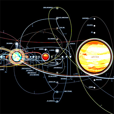


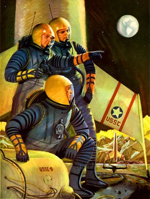
 The main number of interest is deltaV. This means "change of velocity" and is usually measured in meters per second (m/s) or kilometers per second (km/s). A spacecraft's maximum deltaV can be though of as how fast it will wind up traveling at if it keeps thrusting until the propellant tanks are dry.
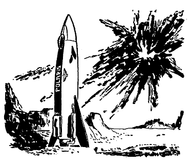
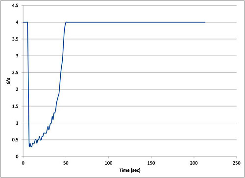


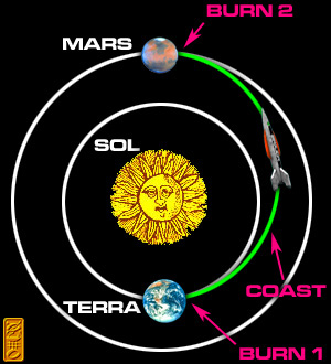
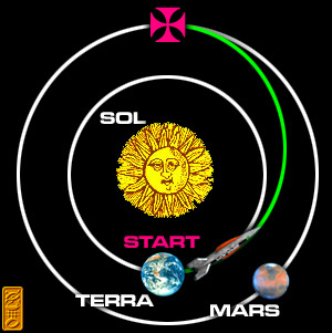
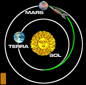
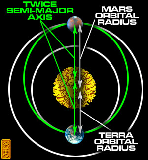
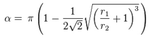
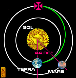

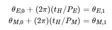
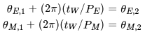
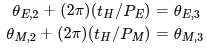
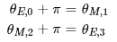
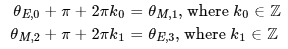

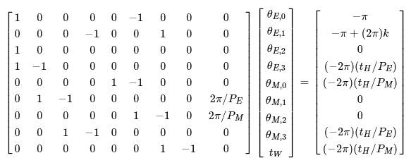
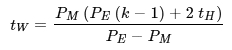
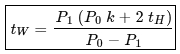
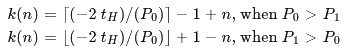
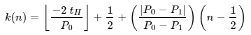
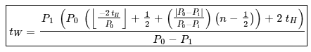
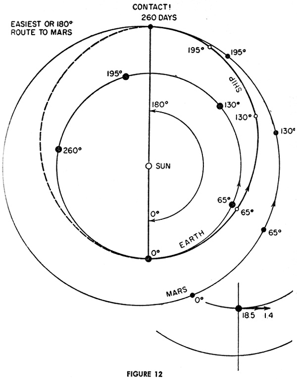
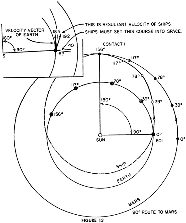
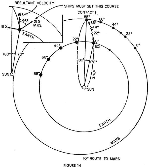
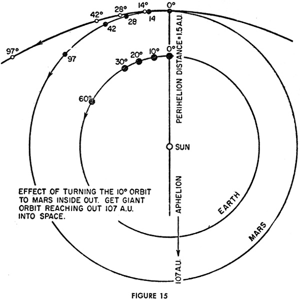
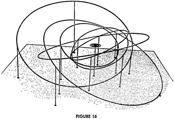
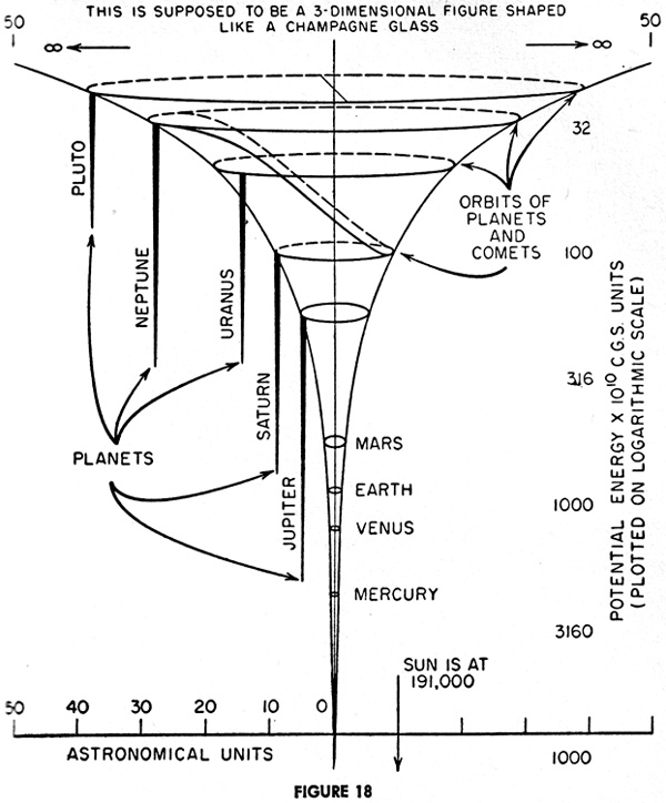
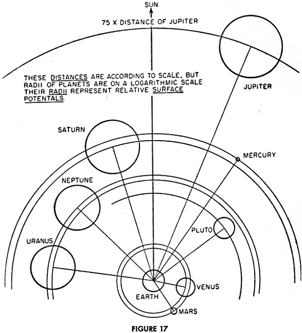


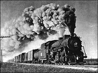
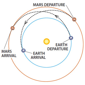
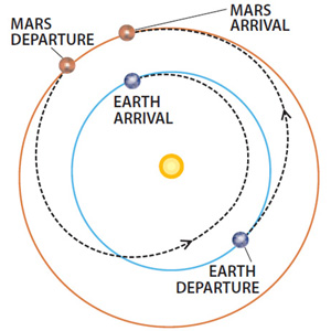
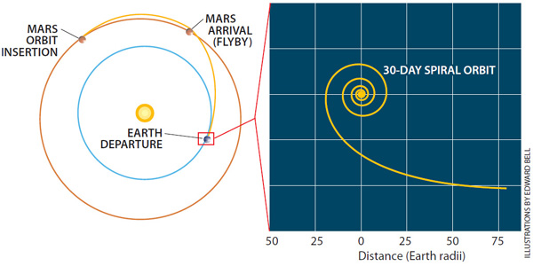


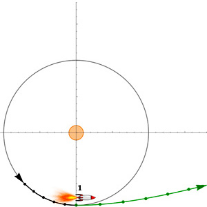
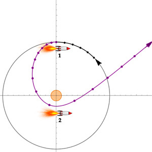
For larger desired values of v∞, the Edelbaum maneuver requires a lower total Δv than the direct or Oberth escapes, and so is fuel-optimal for such high-speed escapes.

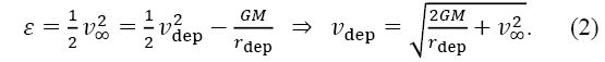


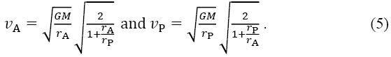

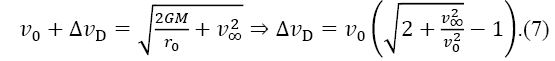
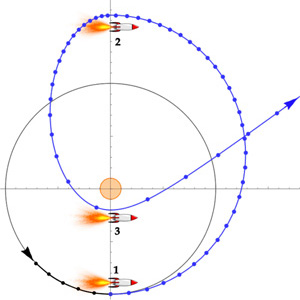
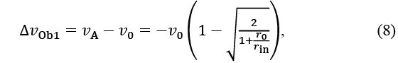
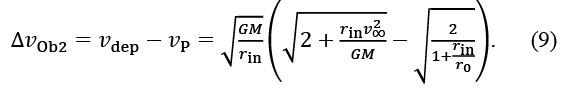
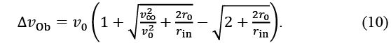
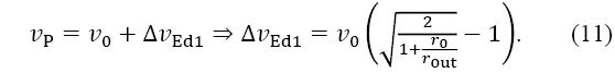
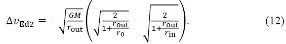
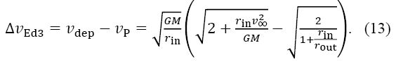
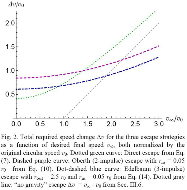
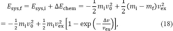
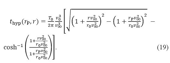
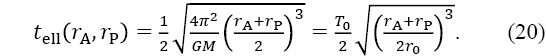
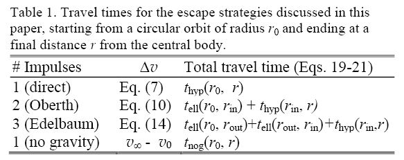
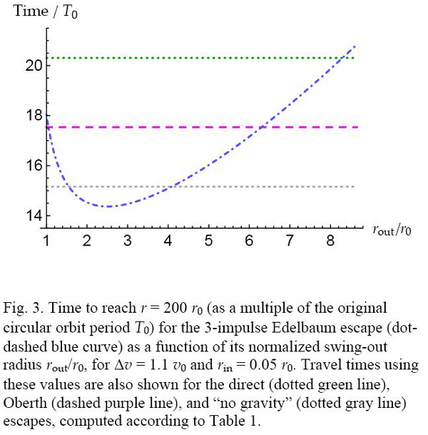
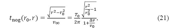
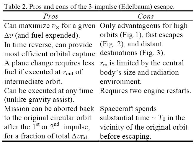


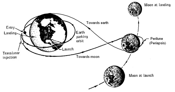

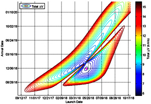


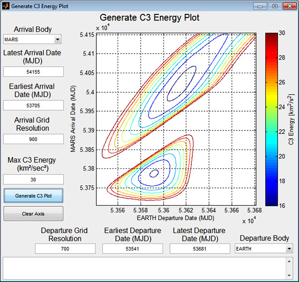
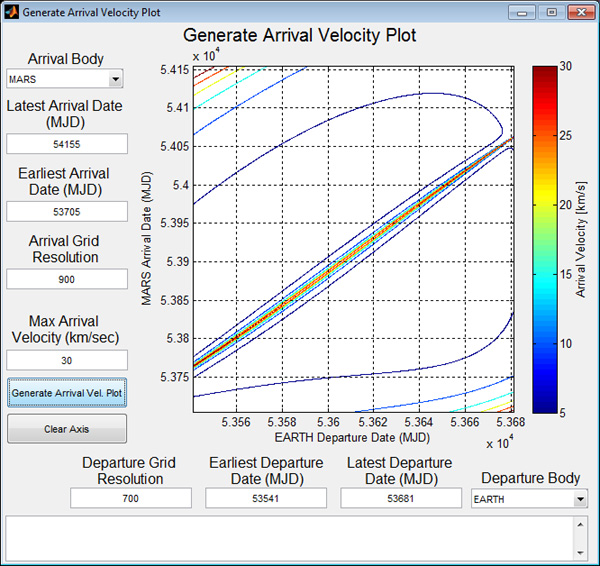

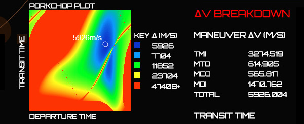


. The principal value of this angle will be between 0° and 180°, inclusive. For now I’ll ignore cases where θ is 0° or 180°. This means that the transfer plane is well-defined and that the number of solutions is finite.